Method proposed for calibrating MFL, UT ILI tools
A new statistical method has been developed and successfully tested for calibrating magnetic-flux-leakage and ultrasonic in-line inspection tools from field verifications.
In contrast to the methods so far available in the literature, the method proposed here can estimate the measurement errors of the ILI and field tools for both constant and nonconstant bias error-in-variables (EIV) models.
The information required to identify the EIV model that describes the comparison of the ILI depth readings with the field measurements can be easily derived from the sizing accuracy claimed for the ILI and field tools. New ILI-tool rejecting criteria are proposed, and it is shown that to reject an ILI run, the measurement errors of the field tool have to be taken into account because they play a key role in computing the number of tolerable bad points in the ILI-field depth plot.
Following the results obtained in this work, the optimum number of field verifications to be conducted is about 30. For this two-tools-one-measurement-each case, the most accurate results are obtained when both tools show similar precision.
In-line inspection
Today ILI tools used to detect, locate, and size such pipeline anomalies as dents, cracks, and corrosion metal loss are based on magnetic flux leakage (MFL) and ultrasonic (UT) principles.1 The information provided by ILI tools consists of geometrical data describing each detected anomaly, e.g., its length, depth, width, and orientation. This information is affected by built-in measurement errors, both systematic and random, that must be considered when the ILI data are used to conduct integrity studies and fitness-for-purpose investigations.2
This article considers only two components of measurement errors: accuracy and precision.
Accuracy refers to the ability to measure the value correctly on average so that it accounts for such systematic errors as constant and nonconstant bias.3
Precision, on the other hand, is a measure of the inherent variability in the measurements so as to account for the random errors that affect the tool readings.
Pipeline integrity analysts and ILI vendors are now aware that, in assessment of defect severity, the key issue is how accurately its geometry has been measured. In this sense, the two important parameters that ILI vendors provide are the probability of detection and the sizing accuracy or measurement errors of the tool.
The measurement errors associated with ILI tools are quoted uniquely as a two-sided confidence interval for a given confidence percentage so that systematic errors are always banned by ILI vendors. The depth-sizing variability associated with corrosion metal loss of today's high-resolution MFL tools is typically claimed to be ±10% WT with a confidence level of 80%, while extra-high-resolution MFL tools are capable of attaining a sizing variability of ±5% WT at 80% confidence.
In the case of ultrasonic tools, high resolution and extra-high-resolution ILIs are claimed to have a sizing variability of ±0.6 mm and ±0.3 mm at a confidence level of 80%, respectively.1
Pipeline operators assess the accuracy of an ILI through the statistical comparison of the metal-loss sizes predicted by the ILI tool with the sizes obtained through field inspections.
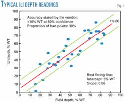
If the accuracy quoted for the ILI tool is achieved during the inspection, then the field vs. ILI depths plot will be fitted to a straight line with unitary slope and about 80% of the comparison points will fall within the sizing tolerance imposed by the confidence level quoted for the tool.
In many practical situations, however, the ILI data are affected by systematic errors in the form of a constant bias (additive error) and/or in the form a nonconstant bias (multiplicative error). Fig. 1 illustrates this latter case for a MFL tool with a sizing variability of ±10% WT at 80% confidence.
Often, analysts assume that the field tool has no errors and estimate the slope of the best fitted line in Fig. 1 using the ordinary least squares (OLS) regression model. It is widely recognized, however, that field instruments, e.g., pit depth gauges, portable UT flaw detectors, laser scanners, and bridging bar systems, show significant measurement errors.
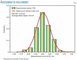
To illustrate this point, Fig. 2 shows the distribution of 178 depth measurements conducted by an experienced field crew member on an internal metal loss using a portable UT flaw detector with 0.025 mm (1/1,000 in.) resolution.
The results of this and other similar experiences conducted using pit-depth gauges and bridging bar systems, have consistently shown that these field instruments show no systematic (accuracy) errors and have associated random (precision) errors that distribute following a normal probability with a variance that depends strongly on the measurement tool type.
For internal metal loss measured with a portable UT flaw detector with 0.025-mm resolution, the 80% tolerance for a single depth reading is about ±0.3 mm.
For external metal loss, this tolerance is about ±0.2 mm for a bridging bar system with a 0.025-mm resolution depth gauge and increases to ±0.5 mm and ±1 mm for pit-depth gauges with 0.4 mm and 0.8 mm resolution, respectively.
Taking into account the sizing accuracy claimed for today's ILI tools, one can conclude that in some particular situations, the measurement errors of the field instrument are comparable or even larger than those of the ILI tool. This situation will arise more likely for ILI runs conducted with extra-high-resolution tools.
If the errors of the field instrument are accounted for, then the OLS regression model is no longer valid to estimate the slope of the best-fit line in Fig. 1, since it cannot distinguish the case in which the ILI-field comparison is affected by systematic errors from the case in which no bias affects the comparison but the field instrument is much more imprecise that the ILI tool.4-6
In such situations, the accuracy and precision of the ILI tool are better estimated with error-in-variables (EIV) models.3 Classical EIV procedures allow dealing with the problem of estimating the slope of the best-fit line in Fig. 1 when both the field and the ILI tools are affected by errors and the ratio of the error variances or one of these variances is known.
In many practical situations, however, the analyst faces the challenge of simultaneously estimating the parameters of the best-fit line and the variance of the errors that affect both tools.
This problem has been addressed in recent publications which focus on the estimation of the variance of the measurement errors of the ILI and field tools using methods available in the literature, such as the Grubbs and Jaech-CELE estimators.4-7 A new Bayesian method, capable of overcoming some of the limitations of these estimators, has also been proposed.6
In these works, however, the bias between the ILI depth readings and the field measurements is assumed to be constant so that the not uncommon situation in which the comparison of ILI with field results obeys a nonconstant bias model has not been addressed yet. In addition, consistent procedures for the statistical calibration of the ILI tools are still missing in the literature.
Calibration model
Calibration determines the scale of a measuring tool based on informative or calibration experiment. Given that field measurements also show error, calibration of the ILI tool is a comparative process.
Click here to view the Equations in PDF.
The calibration experiment obeys Model 13 shown in Equation 1 in the accompanying equations box. The random errors in Equation 1 are assumed to be uncorrelated with dTrue and distributed normally and independently with mean 0 and variance σ2ILI (ILI tool) and σ2Field (field tool). The variable dTrue will be treated as fixed so that Model 1 will be considered a functional relationship.3
The prediction stage of the calibration process is Model 23 shown in Equation 2.
It is noted that the variance of the estimated depth Vˆ(dˆ True)depends not only on the variance of the errors of the ILI tool ôˆ2ILI, but also on the variance of the calibration model. Therefore, it will be always greater than ôˆ2ILI because of the additional (model) error introduced into the analysis during the estimation of the calibration line.
The sampling distribution (dField, dILI) does not allow identification of Model 1 because it is not possible to find a unique relationship between the unknown population parameters and the corresponding estimated parameters.3 Additional information is required to produce consistent estimators of dTrue, aIF, bIF, sILI and sField. The classical EIV procedures can solve the measurement Model 1 only when the ratio of the measurement error variances δ = σ2ILI/σ2Field or one of these variances is known.3
Within the context of the statistical calibration of the ILI tool, however, none of these specifications is available; the classical EIV methods, therefore, cannot be used. Indeed, the sizing accuracy of the ILI tool needs to be corroborated.
In the next sections, a new methodology capable of consistently solving Models 1 and 2 will be described and illustrated using both Monte Carlo simulations and a real-life case study.
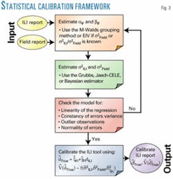
Fig. 3 describes the calibration methodology proposed in this work. Each one of the stages in this figure will be outlined in the following sections.
ILI accuracy
The slope and intercept of the comparison plot are estimated with Wald's grouping method8 in which bIF is found by partitioning the data into two subsets and passing a straight line through the mean points of these subsets. The Wald's estimator of the slope and intercept of the fitted line8 appears in Equation 3.
This estimator is consistent with the true slope in Model 1 if the grouping is independent of the errors and the means of the true values in each group remain different as the number of observations approaches infinity.3 8
This article introduces a modification of the classical Wald's estimator to guarantee that the above conditions are satisfied even if the field readings show large measurement errors.
When it is expected that δ = σ2ILI/δσ2Field ≥ 1, the median of the field readings is used to group the sampling data. Conversely, under the assumption that δ < 1.0, the grouping is done with the median of the ILI readings.
In addition, a robust estimation of mean values in Equation 3 was employed based on an MM estimate9 of the location parameter of each data subset instead of its arithmetic mean. (MM estimates of the regression parameters are robust estimators based on a two-loss function that determines the breakdown point and efficiency of the estimate, respectively.)
It is noted that, in contrast to the classical EIV method, only an estimator of the order of the ratio σ2ILI/σ2Field is required in this modified Wald (M-Wald) method. Table 1 lists the expected range (δ*) for the ratio of the measurement error variance assumed in this work for typical ILI and field tools.
These predictions can be modified to consider other field tools such as laser scanners.
Monte Carlo simulations were used to evaluate the performance of the outlined M-Wald approach with respect to that of the classical EIV method with δ known.
Fig. 4 shows the results of this comparison when δ* < 1.0 for 2,000 samples of 30 comparison points created using the population parameters given in this figure. The performance of the M-Wald estimator is similar to that of the classical EIV estimator, yet it requires only the information given in Table 1 for δ* and not the exact value of δ.
For large measurement errors (σ> 5% WT) and under the assumption that δ*.<.1, however, the EIV estimator proved to perform much better than the M-Wald method. In this particular case, the EIV estimator of the model slope reduces to the classical orthogonal regression estimator, shown in Equation 4.
Precision of ILI, field tools
Several methods are available to estimate the variance of the measurement errors.4-7 For the two-instrument case, one reading by each, the classical estimators are those proposed by Grubbs and Jaech.7 For the nonconstant bias model, the Grubbs estimator can be modified as shown in Equation 5.
In many practical situations, this estimator produces negative error variances. In such cases, the constrained expected likelihood estimator (CELE) proposed by Jaech7 can be used. A modification of Jaech's estimator is proposed in Equation 6 in order to account for the situations where the nonconstant bias model applies (Equation 6).
In Equations 5 and 6, βˆIF is assumed to be 1.0 if the constant bias model is used.
The superiority of the M-Jaech estimators over the estimators available in the literature becomes more evident in situations when systematic errors affect the ILI-field comparison so that βIF.≠ 1.0.
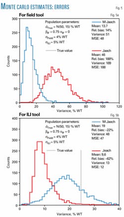
For example, consider a typical situation in which an extra-high resolution MFL inspection is performed on an 11-mm WT pipeline and field verifications are conducted for 30 external metal losses using a 0.4-mm (1/64 in.) depth gauge. In this case, δ* < 1.0 since σField.< 4% WT and σILI < 5% WT.
If additionally it is supposed that the ILI tool underestimated the defect depth and this can be modeled with βIF = 0.75, then the nonconstant bias model will be more adequate to deal with this statistical comparison.
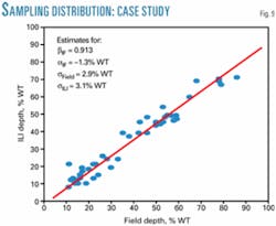
This situation was studied using Carlo simulations for 2,000 samples of size 30. Equation 6 was used to estimate the measurement errors for both the constant (βIF = 1.0) and nonconstant bias approximations. Fig. 5 shows the results of this analysis.
For both tools, the nonconstant bias model (M-Wald + M-Jaech) allows estimation of the measurement error with a smaller bias. Although the constant-bias model produces a smaller variance in the estimation of the ILI tool variance σ2ILI, the bias in this estimation doubles that predicted by the nonconstant bias solution.
Model checks
In this stage, the solution proposed for Model 1 is inspected for faulty conditions such as nonlinearity in the regression, lack of variance homogeneity, outlier observations, and nonnormal distributed errors.
First, the true defect depths and the residuals rˆt from the fitted EIV model are estimated with Equation 7.3
Then, the estimated residuals are plotted against the estimated true depths to check the linearity in the regression and the variance homogeneity postulated in Model 1. The normality of the errors is investigated by plotting the ordered residuals against the expected value of the normal order statistic for a sample of the same size.
The outlier observations are identified with the MM-estimate9 that shows a high breakdown point and an excellent efficiency when the errors have normal distribution.
Calibration of ILI tool
The goal of the prediction stage of the calibration process is the estimation of true value of the metal-loss penetration from the ILI readings. The calibration parameters are estimated with Equation 8.3
If the calibration experiment is carried out with a sample of size n, then the estimator of the true defect depth for the (n+1)th ILI reading and the estimated variance of this estimator are as appear in Equation 9.3
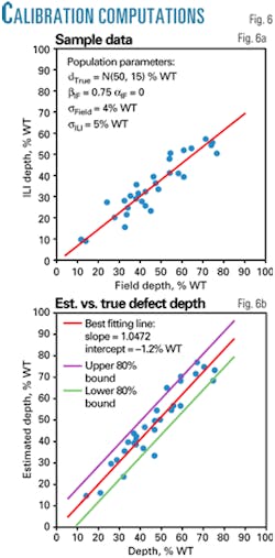
The estimator of δTrue is claimed to be unbiased under the fixed model.3 The variance of the estimated true depth Vˆ(dˆn+1True) is larger than that of the ILI tool σˆ2ILI because it depends not only on the measurement errors but also on the errors introduced into the analysis by the calibration procedure. If γFI is known, then the best estimator of Vˆ(dˆn+1True) is γˆFIσˆ2Field. To illustrate the calibration computations, the typical ILI-field comparison presented in the previous section is considered again. This time, however, the ILI readings are also used as input to predict the true defect depths.
Fig. 6a shows the sampling distribution associated with this comparison, while Fig. 6b shows the regression of the estimated true depths on the actual true depths.
The results presented in Fig. 6b show that Equations 8 and 9 estimate consistently both the calibration line and the true values of the defect depths. The error in the determination of γˆFI, relative to the population parameter γFI, is about 3%, while the OLS regression of dˆTrue on dTrue produces a slope very close to 1.0.
The model variance of the OLS regression is 32% WT. This value is very close to the average variance estimated for dˆn+1True (30% WT) which, in addition, is a larger result than the variance predicted for the ILI tool (16% WT), as expected.
On the other hand, the number of points that fall outside the 80% tolerance bounds (CI80 = ±1.28γFIσˆ2Field) is 5. On the assumption that the number of points that fall within CI80 follows a binomial distribution with n = 30 and P = 0.8, the confidence in rejecting this experiment is 40%, which confirms the validity of these computations.
These results were confirmed using 2,000 Monte Carlo simulations. The calibration slope γFI, the slope βols of the OLS regression of dˆTrue on dTrue, and the model variance of this regression were estimated to be, respectively, (γˆFI)=1.338.6.0.006, (βˆols)=1.004.6.0.002, and (σˆ2ols)=38.3.6.0.6 at 95% confidence. In addition, the confidence in rejecting the calibration experiments was 76% or less, 80% of time.
ILI tool rejection criteria
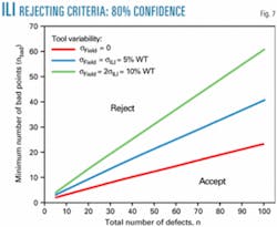
When numerous field verifications are done, the tolerable number of bad points nbad in the ILI vs. field depths plot can be predicted under the assumption that the successful verifications show a binomial distribution. A success is defined as a point that falls within the accuracy tolerance quoted for the ILI tool.
If ps denotes the confidence level used to establish this tolerance and prej the confidence required to reject the inspection, then nbad can be found with Equation 10. This equation assumes that the field tool shows no errors.
If the errors of the field instrument are to be considered, then the value of ps must be modified to reflect the effect of the field measurement errors σ2Field on nbad. The new confidence level ps* to be used in the expression for the minimum number of allowable bad points nbad appears in Equation 11.
In addition, the tolerance range ΔΘ associated with a given confidence level Θ can be found with Equation 12.
Obviously, ps* < ps when δ'-1.≠0, since the errors of the field tool increase the scatter of the comparison points relative to the scatter obtained when σField = 0. Accordingly, a larger number of bad points can be tolerated if the errors of the field tool are taken into account.
Fig. 7 shows this, where the dependence of nbad on n is computed with Equation 11 for δ'-1 = 0, δ'-1 > 1 and δ'-1 < 1 under the assumption that the confidence in rejecting the ILI tool is 80%.
Influence of verifications
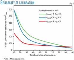
The influence of the number of conducted field verifications on the reliability of the proposed calibration approach was assessed using Monte Carlo simulations for three different populations: {dTrue.< N(50,15)%, βIF = 1.0, αIF = 0} with (σField, σILI) = (3%, 8%), (4%, 5%), and (8%, 2%) WT. In each case, 2,000 experiments were performed for different sample lengths (n = 10, 20, 30, 50, and 100). The mean square error MSEVˆ associated with the estimated variances Vˆ(dˆn+1True) was computed in each experiment from the bias and variance of the estimations.
Fig. 8 shows the dependence of MSE<Vˆ on the number of field verifications. The optimum number of field verifications to be conducted is about 30. If the sample length drops below this figure, the estimation errors increase significantly.
On the other hand, the quality of the calibration does not increase considerably if the number of field verifications is larger than 30. In addition, Fig. 8 also suggests that the most accurate estimations are produced when the errors of the ILI and field tools are similar.
Application
A 36-in. OD, 11-mm WT oil pipeline was inspected with a high-resolution UT ILI tool with 80% tolerance of ±0.6 mm (±5.4% WT). A total of 829 external and 101 internal metal losses were detected, located, and sized.
To calibrate the ILI tool, technicians measured 47 external metal losses at dig sites with a pit gauge with 0.4-mm resolution. Fig. 9 shows the ILI readings against the field measurements. A first computation cycle allowed identification of Point A as an outlier observation.
In a second run, the solution listed in this figure satisfied all the assumptions in Model 1. No reasons were found to reject the linearity for the EIV regression Model 1 or the normality of the errors (the K-S statistic for the test of normality produced a significance level of 0.11).
The underestimation associated with this ILI run was modeled through a nonconstant bias with βˆIF = 0.913 and αˆIF = –1.3% WT. The ratio of the estimated measurement error variances was found to be close to 1.0. This value agrees with the predictions given for δ in Table 1.
In contrast, the constant bias solution with a relative bias of –3.3% WT produced a ratio of 0.3, which strongly disagrees with the expected value for &3948;.
This could be misinterpreted and claimed that the sizing accuracy of the ILI tool is much better than that claimed by the vendor. Based on the evidence provided by Fig. 9, the reasonable conclusion is that the ILI tool performs as quoted with respect to the random measurement errors while a nonconstant bias affects its readings.
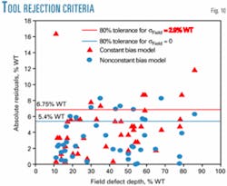
The rejection criterion discussed before was applied to find the degree of confidence with which the ILI run can be rejected. Fig. 10 presents the results of this analysis.
Assuming that the constant-bias model applies and sField = 0, the number of bad points at 80% confidence (±5.4% WT) is 13. This means that the confidence in rejecting the ILI inspection is as high as 87% when this simple model is used.
In contrast, if the nonconstant bias solution is assumed and the outlier observation A is dropped, the generalized rejection criterion gives a 80% tolerance of ±6.7% WT, which reduces the number of bad points to 6. This time, the confidence in rejecting the ILI run is only 8%.
Once the population parameters in Model 1 are consistently estimated, the prediction of the true depth can be carried out for the rest of the defects in the ILI report. In this example, the calibration parameters were estimated to be γˆFI =1.103 and αˆFI =1.4% WT while the average value of the estimated variance of the predicted true depths was determined to be 12.3% WT.
Therefore, the true defect depth associated with each ILI reading was calculated with dˆTrue = 1.4+1.103dILI and a variance of 12.3% WT was assigned to each one of the predicted true depths.
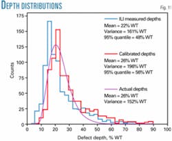
Finally, Fig. 11 shows the distributions of the ILI readings and the calibrated defect depths for the 782 external metal losses found in the inspected pipeline. For the sake of simplicity, they are not corrected for the probablity-of-detection factor.
In agreement with the previous results, the distribution of the predicted true depths is shifted to the right as a result of the underestimation produced by the ILI tool and shows a larger spread than the ILI readings.
The best fitted probability distribution for these histograms were LogNILI(22, 13) and LogNTrue(25, 14), where LogN(μfit, σfit) refers to the log-normal distribution with mean μfit and standard deviation σfit.
How these results are used depends on the approach used to perform the probabilistic risk assessment of the pipeline. For instance, suppose that the failure probability of a pipeline segment is to be computed based on a "typical" defect whose depth attribute is defined through the distribution of the depths of all the defects in the pipeline.
In such a case, the depth distribution to be used is the same as that which best fit the ILI readings with variance σˆ2fit – σˆ2ILI and mean determined by the measurement model selected. Fig. 11 also shows the actual defect-depth distribution predicted from the ILI readings assuming a nonconstant bias model.
On the other hand, if the failure probability of the segment is to be computed with defect attributes that are defined separately for each defect, then the depth value and variance to be assigned to it are those predicted with Equation 9, i.e. δˆn+1True and Vˆ(dˆn+1True). Compared with the previous "distribution" approach, this "direct measurement" method is much more accurate in predicting the segment's failure probability because it allows the most critical defects in the tail of the measured and calibrated depth distributions to be taken into account.2 10
Acknowledgment
This work was done under the collaboration agreement between Pemex-PEP-RS and the Instituto Politécnico Nacional. The authors thank Pemex for permission to publish this article.
References
1. Tiratsoo, J., Pipeline Pigging & Integrity Technology, Houston: Clarion Technical Publisher, 2003.
2. Caleyo, F., Hallen, J. M., González, J, L., and Fernández-Lagos, F. Pipeline Inspection–1: Reliability based assessment method assesses corroding pipelines, OGJ, Jan. 13, 2003, p. 56.
3. Fuller, W. A., Measurement Error Models. New York: John Wiley & Sons Inc., 1987.
4. Bhatia, A., Morrison, T., Mangat, N. S. Estimation of Measurement Errors. Proc. IPC-1998. ASME International. Vol. 1, pp. 315-325.
5. Morrison, T. B., Mangat, N. S., Desjardins, G., and Bhatia, A. Validation of an in-line inspection metal loss tool. Proc. IPC-2000. ASME International. Vol. 2, pp. 839-844.
6. Worthingham, R. G., Morrison, T. B., Mangat, N. S., and Desjardins, G. J., Bayesian estimates of measurement error for in-line inspection and field tools. Proc. IPC-2002. Paper 27263.
7. Jaech, J. L., Statistical Analysis of Measurement Errors. New York: John Wiley & Sons, 1985.
8. Wald, A., The fitting of straight lines when both variables are subject to error. Annals of Mathematical Statistic, Vol. 11 (1940); pp. 284-300.
9. Yohai, V. J., High breakdown point and high efficiency robust estimates for regression. The Annals of Statistic, Vol. 15 (1987). pp. 642-656.
10. Caleyo, F., González, J. L., and Hallen, J. M., A study on the reliability assessment methodology for pipelines with active corrosion defects. Intl. J. Pressure Vessels & Piping, Vol. 79 (2002), pp. 77-86.
Based on a presentation to the 16th World Conference on Nondestructive Testing, Aug. 30-Sept. 3, 2004, Montreal.
The authors
Francisco Caleyo(fcaleyo@ email.com) joined the Pipeline Integrity Analysis Group of the IPN in 1999 where he heads a research team involved with the development and application of structural reliability analysis techniques on onshore and offshore pipelines. He holds a BS in physics and an MSc in materials science from Universidad de La Habana, Cuba, and a PhD (2001) in materials science from Universidad Autónoma del Estado de México.
José Manuel Hallen López is a professor of Instituto Politécnico Nacional (IPN), Mexico, and cofounder of the Pipeline Integrity Assessment Group of the IPN. He holds a PhD (1990) in metallurgy by the University of Montreal.
Jorge L. González is a professor at the metallurgy department of the IPN and works in the field of fracture mechanics and pipeline integrity assessment technologies. He founded and heads the Pipeline Integrity Assessment Group of the IPN. He holds BS and MSc degrees in metallurgy from IPN and a PhD in material science from the University of Connecticut.
Léster Alfonso is a postdoctoral fellow at the Instituto Politécnico Nacional. He holds an MSc in mathematical physics from Moscow State University and a PhD (2002) in atmospheric sciences from Universidad Nacional Autónoma de México.
Eloy Pérez-Baruch is maintenance vice-manager at the Gerencia de la Coordinación Técnica Operativa Región Sur, Pemex Exploración y Producción. He holds a BS in industrial chemistry engineering from IPN and an MSc in pipeline management engineering from the Universidad de las Americas, México.
