Method estimates US refinery fixed costs
A new method for estimating US refinery fixed costs is useful for comparing data between different refineries and is based on the market approach that uses comparable sales.
The Uniform Standards of Professional Appraisal Practice requires the consideration, if available, of actual market sales data in appraising a property. Available comparable sales must be analyzed and adjusted to reflect differences in timing, location, quality, and other parameters that influence the value of the comparable property relative to the subject property.
There are at least two methods of analyzing and adjusting comparable refineries’ sales data. The first is the traditional simplified approach that considers recent refinery sales trends and indices commonly used in the industry, such as sales price as a percent of replacement cost and sales price/complexity-barrel.
Another approach, which is used here, considers adjustment factors to recognize the differences between the comparable refineries and the subject refinery.
The adjustment factors provide a way to quantify the differences affecting a refinery’s value relative to the subject refinery.
Market approach
The first step in the market approach is to review transactions and select relevant sales. Comparable sales are chosen to include refineries as similar as possible to the subject refinery. Unfortunately, no two refineries are exactly the same and few refineries are sold in a given time period.
Typically, data for three or four comparable refinery sales are available. The factors considered to adjust comparable sales include:
• Size (capacity). Differences in operating costs are a proxy for this factor. Variable costs are estimated using operating cost estimates derived from the processes in each refinery. Methods in the public domain are used to estimate these costs. Fixed costs are also needed to calculate a refinery’s total operating costs. This article presents a relationship for estimating fixed costs.
• Location. This influences a refinery’s profitability. An indicator of the gross margin of an average refinery is used here. The 5-year moving average of gross margin for each comparable refinery location relative to the subject refinery location results in the adjustment factor to apply to each comparable refinery.
• Configuration. Estimates of the 5-year moving average gross margin for each comparable refinery are used as if each were located where the subject refinery is. These gross margin estimates are used to adjust the comparable refinery sales for configuration differences.
• Timing. One should estimate 5-year moving averages of gross margins for each refinery ending at the date of sale or as-of-valuation date (for the subject refinery.) This captures the profitability differences for different periods of time, which influences the sales price of each refinery.
Each of a comparable refinery’s four factors, compared to each of the subject refinery factors, gives a percentage adjustment applied to the comparable refinery. The sum of all of the factor percentage differences represents the total adjustment that is applied to each comparable refinery sale to put it on the same basis as the subject refinery. The adjusted comparable sales prices are used to arrive at an estimated fair market value for the subject refinery.
Methodology
To determine an equation for estimating refinery fixed costs, we used fixed cost data from various refinery studies. Refinery fixed cost data included employee expenses, supplies and rentals, repair and maintenance expenses, environmental expenses, insurance, professional expenses, and plant general and administrative.
Property taxes were excluded because this cost is a function of a refinery’s fair market value, which is the result of the appraisal and can vary from jurisdiction to jurisdiction. In practicality, we could have included property taxes in the fixed costs without materially affecting the results, but they were excluded from the data we used.
The data were correlated with variables such as capacity, complexity, location, and type of crude processed.
Variables
There were a total of 12 refineries represented, 4 from US Petroleum Administration for Defense District (PADD) II, 5 from PADD III, and 3 from PADD V, with various numbers of annual observations for each refinery. These explanatory variables were included in our analysis:
• Refinery type: light sweet, heavy sweet, light sour, or heavy sour crudes processed.
• Location: PADD II, PADD III, and PADD V.
• Year of reported costs: 1991 and 1994-2002, inclusive.
• Refinery capacity.
• Refinery Nelson Complexity Index.
Sour crude contains more than 0.5% sulfur and light crude has a gravity of 33° API or greater. A refinery that processes crude with more than 0.5% sulfur and a gravity less than 27° API is a heavy sour refinery.
The PADD II refineries included were in Kansas, Illinois, and Ohio. The refineries in PADD III were all on the US Gulf Coast. All the PADD V refineries were on the US West Coast. There were no refineries in PADD I or PADD IV in the analysis.
Refinery capacities were from Oil & Gas Journal’s refining surveys for the year corresponding to when the fixed costs were observed. Refinery capacities were in b/cd.
The Nelson Complexity Indices were based on published factors (OGJ, Mar. 18, 1996, p. 74). A separate regression included different complexity indices that incorporated some processes not included in the Nelson Index. The results were slightly better because differences between refineries were more completely represented by the indices. The Nelson Index was used in this analysis because it was publicly available and the other indices were not.
Dummy variables, containing either a 0 or 1, were used to represent refinery type, location, and year of reported costs. If a refinery processes primarily light sweet crude, for example, the light sweet variable was set equal to 1 and the other types were set equal to 0. If the refinery processes a different type of crude, the value of the light sweet variable was set at 0.
Similarly, if the refinery was in California, all location variables were set at 0 except the value in PADD V, which was set equal to 1 for that refinery.
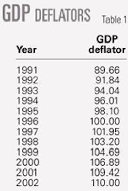
Fixed costs were adjusted for general inflation using the GDP implicit price deflator and were expressed in terms of 1996 dollars.
Table 1 shows the GDP deflator values used in this analysis.
The deflators were used to set a common basis for the fixed costs. If, for example, a refinery had fixed costs of $200 million in 1991, the conversion factor to convert 1991 fixed costs to 1996 dollars was the 1996 deflator divided by the 1991 deflator, 100.00/89.66 = 1.1153. The 1991 fixed costs were therefore $223.065 million in terms of 1996 dollars.
Each of the refinery fixed costs was similarly converted to a 1996 basis before being included in the analysis.
Statistical analysis
A linear regression that used the least-squares method was used to analyze the data. Refinery fixed costs ($1,000/year), refinery capacity (b/cd), and refinery Nelson Complexity Index were transformed into natural log variables. We found that the log relationships fit the data better than the nonlog relationships.
The dummy variables were not transformed because the coefficients associated with these shift variables take the form of the dependent variable. Because the dependent variable was the natural log of refinery fixed costs, therefore, the coefficients of the dummy variables were also natural log values.
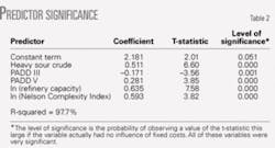
Initially, all the variables were included in the analysis. The data analysis showed that only heavy sour, PADD III, PADD V, refinery capacity, and refinery Nelson Complexity Index were significant variables for estimating refinery fixed costs. A variable was considered to be significant when its coefficient estimate was statistically different from 0.
Table 2 shows the results of the regression with the significant variables and an intercept estimate.
All of the variables in Table 2 were highly significant, i.e., they had a significant influence on observed refinery fixed costs. The overall regression explained 97.7% of the differences in observed refinery fixed costs. For refineries in PADD II, III, and V, therefore, the regression equation accounted for 97.7% of the differences in the observed fixed costs.
Regression equation
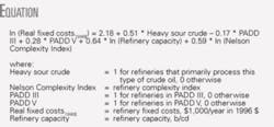
The regression equation (see attached box) provides a basis for assigning fixed costs to refineries used in the comparable sales approach. The range of complexity barrels in the analysis was about 400,000-3 million.
The accuracy of the equation may be lower for refineries whose complexity-barrel values are significantly outside of this range.
This is a common measurement used to describe refineries. It is computed by multiplying the capacity of the refinery (b/cd) by the complexity index. The regression equation contains an approximation of this because ln capacity + ln complexity represents the product of these variables. The regression, however, assigns slightly different coefficients to these variables and, therefore, the sum is not strictly the product of the two (OGJ, Apr. 18, 2005, p. 50).
There were no refineries in PADD I or IV in this analysis. Fixed-cost estimates for refineries in these PADDs are less certain than results obtained for refineries in the other PADDs.
We did not adjust the equation to remove differences that existed due to the structure of the company. The general and administrative expenses, for instance, associated with a refinery contained in a small company may differ from those allocated to a refinery in a large corporation.
To apply this equation, one needs to know the refinery location (PADD), if the refinery primarily processes heavy sour crudes, the refinery capacity, and refinery Nelson Complexity Index. If the refinery is in PADD III or PADD V, the appropriate variable is set at 1, the other is set equal to 0. If the refinery is not in of these PADDs, set both variables equal to 0.
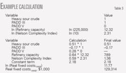
If the refinery processes heavy sour crudes, set this variable equal to 1. If it processes other types of crudes, set this variable equal to 0. The natural log of the refinery’s capacity and the natural log of the refinery’s Nelson Complexity Index are factored by the appropriate coefficients (0.64 for capacity and 0.59 for complexity). The result is the natural log of the estimated fixed costs in thousands of 1996 dollars.
Table 3 shows an example calculation assuming a US Gulf Coast (PADD III) refinery that processes heavy sour crude, has an average capacity of 225,000 b/cd and a Nelson Complexity Index of 10.
If the year of the valuation is 2002, then fixed costs in 2002 dollars are calculated with data from Table 1:
Fixed costs, 2002 dollars = $129.314 million * 110/100 = $142.246 million.
The regression equation is a rule of thumb used when the actual fixed costs of a refinery are unknown. It provides a consistent way of estimating fixed costs for comparable sales analysis adjustments. ✦
The author
Robert Neumuller (Rneu349 @aol.com) is an independent consultant, Plano, Tex. He has 28 years’ experience in the refining and energy industries and has also served as a consultant for Muse Stancil & Co., Arthur Consulting Group Inc., and CPN Consultants Inc. He previously held positions with Southern California Gas Co. and Phillips Petroleum Co. Neumuller holds a BS in chemical engineering from the University of Maryland, an MA in economics from Ohio State University, and an MBA from the University of Southern California. He is a member of the American Society of Appraisers and the National Association for Business Economics.
