Of the total number of wells globally to use artificial lift, 40% employ sucker rod pumps. Pump optimization generally follows established rules of thumb. More advanced pump features, such as pump off controllers (POC) and variable speed or variable frequency drives (VSD and VFD, respectively), require new operating procedures to improve production.
POCs define minimum and maximum pump speeds and implement downtime intervals to maximize pump fillage and minimize pump wear. The POC primarily controls pump speed or frequency by adjusting the strokes per minute (SPM) setpoint of the VSD or VFD. The POC controller will, for example, reduce SPM if pump fillage (PF) drops below a given initial setpoint to avoid pump shutdown. Setpoints are defined at installation and may not be optimized for initial well conditions. Without real-time control, the POC cannot optimize setpoints or adapt to changing conditions.
Speed settings too high or too low result in premature pump wear or suboptimal production, respectively. With increased edge computing and cloud-based connectivity in oilfield operations, new automation programs expand pump performance beyond POC set points for real-time pump optimization. These optimizations are for each well, but control architecture can also optimize overall field performance.
SLB and ExxonMobil Corp. used machine learning tools combined with cloud-based monitoring to optimize production for US unconventional wells requiring artificial lift. The SLB Production Optimizer (PO) algorithm resulted in a 15% overall estimated production increase, and the ExxonMobil machine learning (ML) workflow improved production by an overall 7% while preventing additional compressor failures prevalent with previous manual gas lift adjustments.
SLB production optimization
SLB’s PO algorithm focuses on the PF control setpoint by providing a proportional-integral-derivative (PID) VSD controller function. The autonomous PO workflow uses a rolling window which includes window time (a fixed size of ingested historical data) and period (the duration for the window sliding forward). Windows typically span 7, 14, or 21 days with 4-, 10-, or 24-hr sliding periods. The window ingests well parameters and operational data into the solver to derive optimal frequency setpoints for continuous production optimization.
The ingested parameters include historical pump fillage and SPM data. The dataset is processed for quality and supplemented with pump runtime, shutdown duration, cycle counts, and average pump parameter values.
The algorithm calculates key performance indicators (KPI) for each speed setpoint and recommends an optimum setpoint to maximize production while maintaining pump integrity. Three primary KPIs assess and optimize well performance: Production Indicator (PI), Combined Indicator (CI), and Combined Indicator – Quadratic Penalty (CI-QP).
PI provides a direct relationship between flowrate and speed setpoint to optimize a setpoint that maximizes fluid production. CI quantifies shutdowns on overall production by imposing penalties for shutdown events. A high CI has few shutdowns and higher production, and a low CI could result from lower production, frequent shutdowns, or both. CI-QP includes the same metrics as CI but includes a more severe penalty on shutdowns. This extension identifies excessive cycling to stabilize well production due to the PCS secondary pump fillage setpoint or VFD speed set too high.
The algorithm chooses the KPI based on the best model for the well given production conditions. For example, if the well is overpumping with frequent shutdowns, the CI or CI-QP modes will best address the issue. If a well is underperforming, the PI mode will provide the best approach for production improvement.
Calculated KPIs based on historical speed setpoints produce rolling window KPIs vs. pump operating frequencies. These data produce forecasts for the optimal VFD setpoint in the next window. A forecast where the pump performance trend decreases under increasing pump speed recommends a decrease in VFD frequency by 1 hz below the lowest initial setpoint value. When the performance trend increases, however, raising the pump frequency by 1 hz above the highest setpoint value increases production. In cases where the maximum performance indicator lies within the setpoint median of setpoints, the current frequency setpoint is recommended until the PO determines that the existing frequency no longer provides the optimum production.
SRP optimization deployment
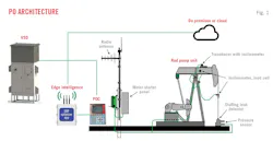
PO deployment requires VSDs for controlling pump speed, a POC to monitor and regulate well performance, and an industrial internet of things (IIOT) edge device for real-time POC communication and surveillance (Fig. 1).
The IIOT captures high-frequency data (per stroke level), but it also can be set by the user at lower frequencies based on bandwidth, storage, or other concerns. The edge device allows both continuous automated and periodic remote manual control over the POC.
PO field testing included eight unconventional horizontal wells in the US spanning a 3-month production period. The algorithm’s optimal set points were manually verified. The tests required that the PO:
- Identify and improve frequent shutdowns and elevated pump failures.
- Identify unattended and underperforming wells.
- Reduce manual interventions that require setpoint changes.
- Optimize pump speed setpoints to achieve optimal pump fillage at lower fluid levels.
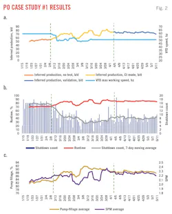
Case Study #1 tested the CI mode because the well exhibited cycling events. The algorithm recommended a reduction in VFD frequency. Fig. 2a shows the well’s inferred production and VFD speed over the course of the test. Inferred production covers historical data (red), model testing and validation (yellow), and post-validation with the algorithm’s chosen optimum setpoint (blue). The PO application produced a 29% increase in inferred production.
Fig. 2b shows the Case Study #1 runtime and shutdown count. Before PO installation, the well experienced 18 daily shutdown cycles. This is why the CI KPI was chosen to optimize well control. During the testing phase shutdown counts decreased to 6-8 times per day and runtime increased 17%.
Fig. 2c shows Case Study #1 average SPM and pump fillage. During the model testing and validation stage, pump SPM and fillage varied until an optimum solution was found. Once the algorithm optimized on 55-hz pump frequency, fillage increased by 7%. Well production was stable after validation with subtle changes in average SPM based on shutdowns.
The well in Case Study #2 was underperforming and nonoptimized, operating at 100% pump fillage with 3.5-SPM pump speed. Because there were very few shutdowns in the well’s history, PO used the PI KPI for well optimization. The algorithm suggested continuous increases in VFD frequency to the maximum available limit of 6 SPM. Runtime remained near 100% with minimal shutdowns. Pump fillage decreased to 90% during the validation period, which was within the acceptable range. Although fillage decreased, the increase in VFD frequency resulted in an overall 35% inferred production increase.
The well in Case Study #3 experienced 85% runtime and 90% fillage based on prior optimization. The well was tested in both CI and PI modes to determine if the well’s performance could improve and select the KPI most appropriate for the well’s conditions. In both cases, the algorithm recommended a reduction in pump speed, with the CI recommendation producing more inferred production than the PI model. Uplift was 8%. Shutdowns were reduced by 46%, indicating that the CI KPI was the most appropriate choice for the well. Runtime increased by 4%, but the reduction in pump speed reduced overall power consumption.
Out of the eight wells tested, six experienced positive improvements. The POC settings could not be modified on one well, and another well experiencing high slugging yielded inconclusive results. Inferred production increased overall by 15%, shutdowns decreased overall by 29%, runtime improved by 3%, pump fillage improved 1%, and SPM increased by 10%. The decreases in shutdowns and SPM increase accounted for the overall production increase even with similar pump fillage to the non-optimized pump history.
ExxonMobil ML gaslift
ExxonMobil developed an automated data-driven ML workflow for gas lift optimization in unconventional fields. The workflow combines an ML model and an optimization framework to forecast the gas lift performance curve and solve for gas lift injection rates subject to field infrastructure constraints.
Gas lift performance curves change during the life of the well, and the optimizer continuously monitors well performance to adjust gas injection rates to maximize production. The ML model relies on historical data training rather than downhole gauge data and multirate testing to determine the best gas lift operating conditions for each well in the field. This approach is ideal for unconventional assets which do not have access to real-time data.
The workflow involves three components: 1) the ML forecaster, 2) a Baysian optimization, and 3) model deployment. The ML model applies to all wells and learns from historical production and gas injection rates to forecast gas-lift performance curves.
ML gas-lift optimization
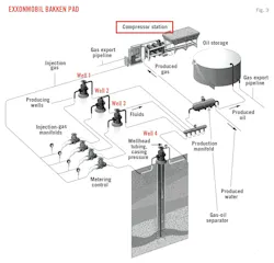
The model was applied to Bakken field which has scarce instrumentation, no downhole gauges, and poor compressor reliability. The field uses pad compression with limited weekly gas rate changes, and these changes result in compressor problems which typically shut down pad production for multiple days (Fig. 3).
The ML forecaster was trained on historical Bakken data which included daily production rates, gas injection rates, and surface pressures. The liquid production typically followed an exponential decay trend. The data were cleaned before applying ML learning by first removing the first few months of data which represent transient effects. This process prevents ML training bias by only training on steady-state data. Additional data removal included flatlines in daily data, weeks with more than 6-hr downtime, days with non-physical (realistic) oil production and gas injection, initial flush-out days following long shut ins, and non-physical surface pressures and temperatures. The data were smoothed in 1-week time windows.
After cleaning, aggregate well data are plotted during production weeks to develop the predictor algorithm. The difference between adjacent week’s production is calculated to convert from a time-based trend to a static difference quantity. The time series problem thus converts to a regression problem to optimize on liquid production. The regression maps temporal features, control parameters, and static features to the target liquid production at a given forecasted week.
The temporal features include rolling time-series surface pressure and temperature during the previous 3 weeks to the target week (Fig. 4). The control parameter is the gas injection rate that will be set at the target week. Static features include lateral length, total vertical depth, acreage area, production age, and other well-specific features.
The ensemble ML model includes simple stacking with Random Forest and XGBooster regressor models and a Kernal Ridge Regression (KKR) model with a second order polynomial kernal. This type of model stacking provides optimum ML models based on the situation to improve forecasting. The Random Forest model, for example, does not accurately extrapolate gas injection rates beyond those contained in the training data, but switching to the regression-based KKR model improves extrapolation (Fig. 5).
The ensemble model is tuned over the range of multiple data parameters taking care not to leak time-based data into the future forecasting time. Training predictions (using 80% of older historical data) and test predictions (using newer 20% hold-out test data) show similar accuracy, verifying the model workflow. Sensitivity analysis showed that the decline trend was the most important parameter for accurate forecasting. The gas injection rate was secondary in importance with pressure and temperature making tertiary impacts.
The forecaster produced forward weekly performance curve optimizations for every well to maximize pad production without exceeding compression capacity. Given relatively minor gas lift changes in real-world systems during multi-week intervals, the model’s predictions filtered through a reality check to ensure that the model did not recommend unrealistic large-scale changes within a week’s time. The forecaster focused only on well performance optimization; local pad infrastructure constraints were not included in the model. This part was handled by subsequent Baysian optimization.
A Baysian optimizer ensured that each pad compressor’s minimum and maximum capacity was honored in the forecast. The constrained optimization workflow included well-to-compressor mapping, the compressor’s capabilities, and gas-lift performance curves from the ML forecaster. The Baysian operator uses past pad history to guide future recommendations. Final optimal gas injection rates maximize total production from all wells sharing the same compressor.
The workflow was deployed to the Bakken asset through the cloud using two continuous-integration continuous-deployment pipelines (CICD) including a training pipeline and a predictive pipeline.
The training pipeline generates a trained ML model. To capture data shift trends (more wells online with gas lift, etc.) the model is retrained every month with the latest available data. The new model is compared with existing models on the same hold-out test set to ensure accuracy. If the new model is more accurate, it gets loaded into the predictive pipeline, otherwise the predictive pipeline uses the existing model.
The predictive pipeline runs on a weekly basis and loads the pre-trained ML model to forecast each well’s gas lift performance curves and solves for optimal gas-injection rates with compressor constraints. The results are pushed to the end user through the dashboard. The predictive pipeline also monitors the ML forecasts by comparing the previous week’s predictions to measurements. Developers are alerted if the deviation between the two is large for several weeks in a row.
Bakken optimization results
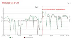
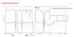
Before full ML deployment, a pilot program tested the workflow on about 30 wells across eight different pads. Uplift was about 5%. Fig. 6 shows results of uplift when the optimizer recommended an increase in gas lift, and Fig. 7 shows results from a different well when the optimizer recommended a decrease in gas lift. The red dash indicates the time of optimizer implementation. Both wells show an increase in uplift, demonstrating the ability of the optimizer to handle different well requirements.
The success of the pilot resulted in a fully deployed workflow in the Bakken for more than 200 gas-lifted and plunger-assisted gas-lifted wells. The first 50 wells optimized resulted in 84% working at near optimal rate without stressing the compressors. Uplift is about 7% on average for these wells. The dashboard has been sending back detailed optimization data to the Bakken team to aid its monthly surveillance and optimization meetings.
Based on “Autonomous SRP Optimization Using and Edge-Based Data-Driven Solution,” SPE-218539-MS, SPE conference at Oman Petroleum & Energy Show, Muscat, Oman, Apr. 22-24, 2024, and “A Machine-Learning-Based Gas Lift Optimization Workflow for Unconventional Fields,” URTeC: 403353, Unconventional Resources Technology Conference, Houston, Tex., June 17-19, 2024.
About the Author
Alex Procyk
Upstream Editor
Alex Procyk is Upstream Editor at Oil & Gas Journal. He has also served as a principal technical professional at Halliburton and as a completion engineer at ConocoPhillips. He holds a BS in chemistry (1987) from Kent State University and a PhD in chemistry (1992) from Carnegie Mellon University. He is a member of the Society of Petroleum Engineers (SPE).
