P. 3 ~ Continued - Dependent on dependence: Are economic calculations of expected hydrocarbon accumulations worthwhile?
View Article as Single page
The point about this situation is that Pc can have any value in between 50%>Pc>0%. When one assigns any value whatsoever to Pc in the allowed range then the expected value of the Fig. 2 decision tree diagram is independent of the assigned value for Pc and is precisely the expected value for the situation where A and B are treated as independent reservoirs. Not only that, but the standard deviation around the expected value is also independent of the value chosen for Pc within the limiting range and is 9.2 million bbl, in agreement with the situation where A and B are taken to be independent when the standard deviation is also 9.2 million bbl.
One aspect of this independence is that one can provide immediately a cumulative probability curve of the chances of exceeding a fixed value, and this curve does not change as the probability dependence is varied. Fig. 2 shows the cumulative probability curve for the parameters of Fig. 1.
A corollary is that if one were to replace Pb in the above argument by any value whatsoever then one would again obtain a range of values for Pc for which there is no change in the expected value or the standard deviation, although the expected value would then be different than for the situation where A and B are treated as independent. In other words, there is a large class of situations for which dependency (either negative or positive) allows no distinction between possible outcomes—this general result has far-reaching implications for a corporation as is discussed below.
A measure of the trustworthiness of the expected value is the volatility, defined as standard deviation divided by expected value. If the volatility is much less than unity then the expected value represents a good assessment of likely worth whereas a volatility much larger than unity informs that the expected value has a large uncertainty and less confidence should be placed in the expected value as a good representation of the worth. For the values reported in Fig. 1 (A and B treated as independent) the volatility is 1.96 while in the dependent case shown in Fig. 2 the corresponding volatility is also 1.96 because both the expected value and the standard deviation are identical.
One of the more useful measures of worth is the cumulative probability, P (>Y), of obtaining a worth exceeding a chosen amount Y. However, one must also ensure that one does not violate the maximum allowed value, obtained when all probabilities are maximized and for which the total available reserves are then 40 million bbl for the example given in Figs. 1 and 2. Hence one writes:
where EV is the expected value and σ is the standard deviation: A is the maximum amount of reserves (for the example A = 40 million bbl).
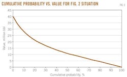
Equation (1) is valid for A>Y>0 so that one has a valid descriptor of the influence of uncertainty on the anticipated worth of the situation including the dependence. Fig. 3 shows the corresponding cumulative probability and value (in million barrels).
Three markers considered of worth in the oil industry are P10, P50, and P90, which are the values of Y corresponding to 10%, 50%, and 90% cumulative probability of greater than the defined value, respectively.
For the example of Fig. 2 these marker values are 28, 11, and 2.2 million bbl, respectively. The three values provide a corporation with an assessment of worth in the sense that a P50 of 11 million bbl indicates there is a 50-50 chance of either more or less than 11 million bbl, while the ratio of |(P90-P50)/(P50-P10)| provides an indication of the anticipated likely dynamic range possible and takes on the value 0.52 indicating there is about a 2:1 bias around the P50 value for assessing likely value, as could also have been obtained directly from the differences in the marker values around the P50 value(11 million bbl vs. 9 million bbl).
It is unlikely that one will obtain less than 2.2 million bbl but equally unlikely one will obtain more than 28 million bbl—estimated at the 10% and 90% probability values.
In addition, because the expected value and the standard deviation are identical for both cases then the cumulative probability curve shown in Fig. 2 is also applicable to the case where both A and B are taken to be independent.
Displaying 3/5
View Article as Single page


