Portfolio optimization benefits from integrating analysis of risk, strategy, and valuation
Optimization of oil and gas assets within a portfolio requires analysis and techniques that go beyond the efficient frontier favored by the traditional portfolio theory developed to optimize stock portfolios.1
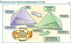
Four numerical techniques, specifically adapted to portfolio analysis, when applied in an integrated manner, provide significant insight to how groups of oil and gas assets can be best combined to form optimum portfolio under strategic constraints. Called here "the four S's," they are:
- Simulation-to quantify levels of uncertainty.
- Statistics-to focus analysis on (downside) risk without limiting (upside) opportunity.
- Simplex-linear program algorithm that converges analysis towards optimum solutions when specific constraints are applied.
- Spreadsheets-driven by macro- code, these form a flexible platform for facilitating the required numerical analysis, with additional advantages of providing access to intermediate data and excellent graphical output.
Given the power of modern computers and the flexibility of standard software packages, calculation of large volumes of simulation data is perhaps the easiest part of process. Careful formulation of the problem and its constraints, strategic or otherwise, is essential in building workable portfolio models that do not overlook key risks or dependencies. The initial model set-up, the analytical and graphical techniques used to compare "optimum" solutions, and the staged approach to risk analysis enable the system proposed here to expand on traditional portfolio theory (Fig. 1).
Risk analysis
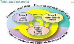
Analyzing risk in a staged manner distinguishes risks at the asset level, the pretax portfolio level, or the post-tax corporate level. The author proposes a three-stage approach to risk analysis.2 3
- Stage 1 (asset-based risk analysis): Perform risk analysis on each portfolio asset individually to quantify its chance of success (technically and economically). Use this to calculate an expected monetary value (EMV) for each asset (a discounted cash flow adjusted by its chance of success). Extend this evaluation with sensitivity cases and probabilistic analysis to verify the viability of each asset on a stand-alone basis. Reject from the portfolio those assets that fail to pass defined hurdles of economic viability. This step distinguishes asset-based risks from portfolio risks.
- Stage 2 (pretax portfolio risk analysis): Apply economic risks as part of a Monte Carlo simulation analysis of the combined portfolio of assets, but consider only those factors that are independent of a specific corporate financial structure. Quantify risk associated with portfolio EMV distributions calculated from simulation runs. Analyze the EMV distributions statistically, and plot value-vs.-risk diagrams for the full portfolio and rationalized combinations of assets. Provisionally identify optimum asset combinations based upon specific corporate constraints, such as capital expenditure and production volumes. Explore which assets are pivotal to maintaining value or contributing risk to the portfolio. This analysis provides a free market value of the portfolio: what a willing purchaser might be prepared to pay for the group of assets.
- Stage 3 (post-tax portfolio risk analysis): Integrate the Stage-2 analysis with a corporate financial model and strategic post-tax performance targets. Extend the simulation to calculate distributions for a number of profit-and-loss and balance-sheet parameters. Analyze the parameter distributions statistically to establish the probability of achieving targets, and quantify risk. Redefine the efficient frontier in terms of post-tax, risked, and discounted corporate cash flow and net income. Stage-3 risk analysis extends the simulation and optimization analysis to incorporate factors such a debt, equity, and tax pools that are specific to the corporation holding the portfolio.
Fig. 2 highlights the need for each stage of the analysis to be revisited on a regular basis for a portfolio model to be used effectively as a management tool to monitor the performance of a group of assets. Information and circumstances can change the relative contributions that assets make to a portfolio through time. As new data become available-such as an oil price forecast or production performance from a specific asset-each Stage of the analysis requires updating. Once a model is built, updating it and testing how new assets fit with the existing asset mix are relatively straightforward.
Linking to targets
Risked values of many oil and gas portfolios conform to skewed diStributions. It is appropriate to distinguish uncertainty on the high-value side of the distribution (opportunity for gain) from uncertainty on the low-value side of the distribution (risk of loss, downside risk, or simply "risk" as used here). Selecting the portfolio with the minimum standard deviation minimizes uncertainty, but in skewed distributions it can confuse risk and opportunity.
Portfolio optimization should focus statistical risk measurements on the low-value side of the risked cash flow distributions generated from simulation models. The semistandard deviation of value outcomes that fall below specified target values is a useful way to quantify risk in this context.4 This is calculated with the following formula:
null
Where, "St" is the semistandard deviation below target value "t," "v" is any value in the distribution with a value less than target value "t," and "N" is the total number of values in the distribution below target value "t."
Another measure of portfolio risk is the probability of a target being achieved (or not) within a value distribution.
These two measures of risk complement each other: The semistandard deviation quantifies the magnitude of risk in the same units as the value distribution itself; the probability of achieving specific values quantifies the chance, in percentage terms, of a portfolio achieving a specific strategic target. A key attribute of both measures of risk is their ability to relate risk to specific strategic targets and not just evaluate the risk of making a profit or a loss.
The balanced-scorecard strategic management system promotes establishing quantifiable strategic goals to which short-term and long-term budgets and individual performance are aligned.5 Numerical portfolio optimization models with risk measures linked to strategic targets provide tools to make this possible and assist in honing strategy.
Optimization software
The traditional portfolio analysis approach, and the driving force behind much optimization software currently used by the industry, is to define an efficient frontier on a value-vs.-risk plot, and then select from among many possible portfolios along the efficient frontier. While this approach is valid (except that many models ignore asset-based risks), it addresses only some of the issues and does not necessarily reveal why certain asset combinations lie at the high-risk end of the efficient frontier and others at the low-risk end.
More detailed analysis of which assets are driving portfolio risk and value is required. The efficient frontier represents the optimum boundary to a feasible envelope of possible portfolios. Defining the boundaries to the entire feasible envelope, in addition to the efficient frontier, reveals a more complete picture to the analyst.
However, most organizations do not have asset portfolios situated on the efficient frontier. There are several reasons why in the real world portfolios lie within the feasible envelope rather than on the efficient frontier. For example:
- Declining or inefficient assets that cannot be easily disposed of.
- Current, suboptimal performance of assets, facilities, or markets.
- Strategic conStraints, such as capital expenditure or production throughput.
While it is clearly important to direct the portfolio towards the efficient frontier, it also is crucial to know where the portfolio lies in relation to other boundaries of the feasible envelope and what effect imposing specific strategic constraints-such as capital expenditure limits-has on that position. No possible combination of assets can by definition lie outside the feasible envelope on a value-vs.-risk plot.
A primary objective for value-vs.-risk plots should be to define the feasible envelope. There are two approaches to doing this: 1) calculating hundreds or thousands of portfolio combinations and placing a boundary around them in value-risk space, and 2) identifying the relative contributions to portfolio value and risk of specific assets or asset groups by removing them in fractions from the portfolio and comparing the effect, then calculating 50 or so extreme points.
The second approach provides the analyst with more insight as to which assets are pivotal in driving portfolio value and risk. The more assets that are involved in a portfolio, and the more diverse those assets are, the more time-consuming this Step of the analysis becomes. However, it is an important analytical step, as the highest independently valued assets may not be the most critical to portfolio value and risk.
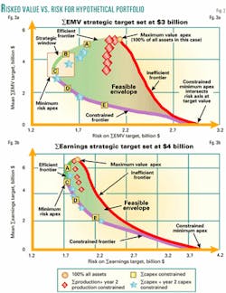
Fig. 3a is a plot of value (ΣEMV, the sum of risked and discounted cash flow for all periods for all assets included in specific portfolio combinations) vs. risk for a hypothetical portfolio on which the feasible envelope is marked. It is useful to study the shape and different boundaries and apexes defined by the envelope as these will vary depending upon the assets involved and the value measures displayed. The width and slope of the efficient frontier are important: The flatter and wider this boundary, the more flexibility and choice are available to reduce risk without significantly compromising value.
If the strategic value target is set at zero (to discriminate profitable from loss-making simulation outcomes) the constrained minimum apex of the feasible envelope passes through the origin of the value-vs.-risk plot. Where the value target is aligned with a strategic objective, the constrained minimum apex (all assets removed from the portfolio) will intersect the risk axis at the target, as all simulation trials will have zero value.
For financial-value variables, the feasible envelope often has the form of a deformed balloon. The maximum-value apex usually contains all assets in the portfolio, assuming no loss-making assets, which should have been culled at stage 1 of the risk analysis if strategically possible. It lies at the upper end of the efficient frontier. As inefficient assets are progressively removed, portfolios plot at positions moving from right to left along the efficient frontier, with small reductions in value accompanied by large reductions in risk.
The efficient frontier steepens at its left end as it approaches the risk-minimum apex-the low-risk, low-value end of the efficient frontier representing an inflection point below which the risk of achieving the target increases. The portfolio combination representing the minimum risk apex will vary depending upon the target value used for the semistandard deviation risk calculation.
The constrained frontier displays the minimum-return portfolio for a given level of risk, and asset combinations situated along this boundary contain relatively few of the high-value assets available. The higher the target value the longer the length and steeper the inclination of the constrained frontier. However, for a given set of assets the shape of the feasible envelope is similar for a range of target values within the limits greater than zero and less than the maximum apex value.
Simplex models
Asset risk analysis, simulation, and downside statistical analysis and modeling asset combinations get us to the point of defining the feasible envelope. Linear optimization techniques (for example, the simplex algorithm6) facilitate the definition of optimum asset combinations within the feasible envelope when specific and, frequently, compound Strategic constraints are imposed.
The squares in Fig. 3a represent the optimum portfolio combinations for various levels of total capital expenditure (ΣCapex represents the sum of capital expenditure for all periods on all assets included in a specific portfolio). The maximum apex portfolio (100% of all available assets in this case) has ΣCapex of greater than $4 billion. Squares labeled A, B, C, D, and E are optimized for ΣCapex of $3 billion, $2.5 billion, $2 billion, $1 billion, and $0.5 billion, respectively. These optimum points for specific budget constraints, selected by the simplex optimizer, lie around the boundary of the feasible envelope.
As constraints become more confining, optimum solutions, if they exist, move away from the efficient frontier boundaries and into the body of the feasible envelope. For instance, the stars in Fig. 3a represent optimal portfolios with a ΣCapex constraint of $3 billion and with an additional constraint on capital expenditure in year 2 of the planning horizon, varying from $700 million progressively down to $50 million. The trend starts at the point on the efficient frontier where the $3 billion ΣCapex constraint applies and moves into the body of the feasible envelope through constrained portfolios as the year-2 constraint becomes more severe. The trend rejoins the feasible envelope at the risk-minimum apex when the year-2 constraint is $200 million and becomes the controlling constraint. The trend continues down the constrained frontier for lower limits on year-2 expenditure.
The diamonds in Fig. 3a display another example of multiple constraints leading to optimal portfolios within the body of the feasible envelope. Here there is a constraint that ΣProduction must be above 500 million bbl and an additional constraint that production in year 2 is limited (perhaps for operational reasons or facilities constraints) to varying levels between 60 million bbl and 30 million bbl. The simplex algorithm optimizes ΣEMV with these constraints, which as they become more severe move the optimum portfolio further from the efficient frontier.
The simplex method offers a rapid and effective means of modeling the impact of constraints within the feasible envelope. Linear optimization should not, however, be used in isolation of risk-analysis techniques to select an optimum portfolio. Risk does not behave linearly and requires simulation and statistical analyses to define it. The simulation-simplex combination is, however, a powerful tool for integrating risk, value, and strategy analysis and optimizing the results. It enables a strategic window to be placed on the risk-vs.-value plot (Figure 3a), which can then be studied for fine-tuning the selection of the optimum portfolio within the prevailing constraints
Value-vs.-risk diagrams should not be limited to risked and discounted cash flow metrics. Risked and discounted earnings is an important value metric to study as the strategy of many organizations is to maximize earnings and not cash flow. Fig. 3b shows the Σearnings-vs.-risk diagram and feasible envelope for the same set of hypothetical assets with a $4 billion Σearnings target. The feasible envelopes for EMV and earnings usually have different shapes, and specific asset combinations lie at different positions within them. The earnings efficient frontier is shorter and steeper, which means that any constraints will significantly reduce value for relatively small reductions in risk.
It is important to compare the feasible envelopes for different value measures and to optimize with the values that are aligned with corporate objectives. It is pointless to set the objective function of the simplex optimizer to cash flow when the corporate strategy is to maximize earnings.
Honing targets
Once the feasible envelope is established and the simplex model has identified optimum combinations within a strategic window, there is more information within the statistical analysis of the simulation data that can help in the portfolio selection process. Testing and comparing the ability of asset combinations to achieve specified strategic targets for a range of key metrics can be very revealing and also can help to hone strategic targets. For oil and gas assets, obvious metrics to study are production and capital expenditure metrics together with finding and development costs; depletion, depreciation, and amortization; and other dollar-per-barrel metrics.
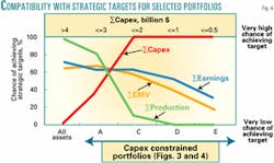
Fig. 4 displays a line plot synthesizing analyses for four key metrics for five portfolios spread around the feasible envelope. It reveals their ability to meet some but not all of the strategic targets.
The maximum value portfolio (100% of all assets) is almost certain of achieving the strategic production target but equally certain of breaching the strategic capital-expenditure limit. It has a 65% chance of achieving the EMV and earnings targets. The uncertainty is due to the ranges input to the simulation (in this case a wide range of future oil prices is the main contributing factor to risk). Other portfolios can almost certainly achieve the capital-expenditure target but in doing so will almost certainly fail to meet the production target but not significantly increase the risk of failing to achieve the EMV or earnings targets.
At this stage of the analysis it may be necessary to verify or redefine strategic targets to make sure that they are mutually consistent and achievable. The targets can then be used as meaningful performance measures.
An integrated simulation-simplex approach offers the portfolio manager flexibility to interrogate the available data interactively to narrow down the feasible options for asset combinations that optimize risk, strategy, and value.
References
- Markowitz, H.M., "Portfolio selection," Journal of Finance, Vol. 7, March 1952, p. 52.
- Wood, D.A., "Three-Stage approach proposed for managing risk in exploration and production portfolios," OGJ, Oct. 23, 2000, pp. 69-72.
- Wood, D.A., "Three Stages of Risk Analysis: Improving E&P Portfolio Management and Its Links to Corporate Strategy," OGJ Executive Report, Penn- Well Corp., 2000.
- Orman, M.M., Duggan, T.E., "Applying modern portfolio theory to upstream inveStment decision making," Journal of Petroleum Technology, March 1999, pp. 50-53.
- Kaplan, R.S., Norton, D.P. "Putting the balanced scorecard to work," Harvard Business Review, September-October 1993, pp. 135-142.
- Dantzig, G.B., "Linear Programming and Extensions," Princeton University Press, 1963.
The author
David A. Wood is an exploration and production consultant specializing in the integration of technical and economic evaluation with management and acquisitions Strategy. He also provides an extensive range of training on upstream economics, international fiscal terms, risk and portfolio analysis, and is a director of E&P management courses with the College of Petroleum Studies (Oxford, UK). After receiving a PhD in geochemiStry from Imperial College in London, Wood conducted deep sea drilling research and in the early 1980s worked with Phillips Petroleum Co. and Amoco Corp. on E&P projects in Africa and Europe. During 1987-93, he managed several independent Canadian E&P companies (Lundin Group), working in South America, the Middle EaSt, and the Far EaSt. During 1993-98, he acquired and managed a portfolio of onshore UK and North Sea companies and assets as managing director for Candecca Resources Ltd. Wood is the author of four Oil & Gas Journal Executive Reports on risk analysis and related subjects (for information, contact Linda Barzar at 713-963-6229; email: [email protected]). His e-mail address is [email protected].


