Learn strengths, weaknesses to understand Hubbert curve
M. King Hubbert was a distinguished scientist published on many aspects of petroleum geology, but he is most remembered for his 1956 work on forecasting production in which he introduced a special bell curve that bears his name.
Hubbert was also remarkable for his interest in the social implications of resource depletion.
In 1974,1 he presented several production curves for the world and the US but was somewhat reticent in explaining the mathematical basis of his work. He referred to a bell-shaped curve, of which the most commonly used are the normal or Gauss curve, and also to the derivative of the logistic curve,2 but he gave no equations. He based his study on ultimate recovery, taking 170 billion bbl for the US and low cases and high cases for the world of 1,350 billion bbl and 2,100 billion bbl, respectively.
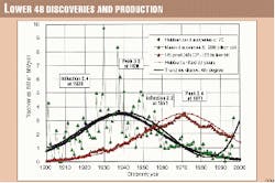
His initial study concerned the US Lower 48 states, which had a single cycle of continuous exploration in a large number of basins. He referred also to the relationship between discovery and production. The discovery cycle peaked in the late 1930s and was followed by a corresponding production cycle peaking around 1970.
But as explained below not all countries are characterized by a single discovery cycle; other constraints to the Hubbert model need to be better understood. It is to be noted in particular that the model is a symmetrical curve, whereas the production curve of an individual field is generally asymmetrical. As discussed below, the Hubbert curve is in fact the derivative of a logistic curve.
Constraints
A simple Hubbert curve may be ideally applied only in the following cases:
- Where there is a large population of fields such that the sum of a large number of asymmetrical distributions becomes symmetrical (normal) under the Central Limit Theorem of statistics. There are several examples of inadequate populations, as Illinois and Ohio with few fields (highlighted by McCabe3 in his criticism of Hubbert) or Alaska and the North Sea, where a few giant fields came on production simultaneously when the pipeline connections were made.
- Where exploration follows a natural pattern unimpeded by political events or significant economic factors, as for example when OPEC artificially cut production: Hubbert modeling should not be used for the swing producers (Persian Gulf).
- Where a single geological domain having a natural distribution of fields is considered, political boundaries should be avoided.
Hubbert himself did not appreciate these constraints since he worked on the US Lower 48 and the world as a whole, prior to significant OPEC intervention.
Methodology
It is well to remember at the outset that what is born must die: even the sun and our planet have a life ending in death. What goes up must come down.4
Biological growth starts with an exponential multiplication (1-2-4-8-16ellipse) as each cell divides, but because of constraints (mainly space and family planning for human beings) growth declines and population reaches a maximum and declines to death. Ultimately nothing is linear, least of all producing a finite natural resource formed but rarely in the geological past.
The classic logistic curve was discovered by Verhulst in 1845 in connection with population studies. It was used to propose that population growth increases to a midpoint (tm) and then decreases to zero, giving what is known as an S-curve. In this application, where there is no negative growth, total population stays constant at the asymptote (U). In the 1920s Pearl and Reed used the logistic curve to model the US population.
It can also be used in modeling oil cumulative production under the formula
Q = U/1+EXP(b(t-tm))
where t is the reference date (year), Q is cumulative production at the reference date (t), U is ultimate recovery, tm is the date at midpoint, and b is a factor describing the slope.
But in practice it is more convenient to use the derivative of the logistic curve to model how annual production starts and ends at zero with a peak in between. It is in effect the Hubbert curve, although there are variants such as the Gauss curve, the Cauchy curve, the sine wave, and even the parabola. These alternatives give similar results for the upper part of the curve, which is the more important part, but the Hubbert curve is the easiest to construct using one of the following formulae:
P = 2Pm/(1+COSH(b*(t-tm)), or
P = 2Pm/(1+COSH(5(t-tm)/c)), or
P = 2 Pm/(1+COSH(6(t-tm)/d)).
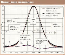
COSH is the hyperbolic cosine equaling (EXP(x) + (EXP(-x))/2) where (Fig. 1)
P is annual production (= dQ/dt),
Pm is production at peak (midpoint of ultimate),
tm is the year of peak (at half life),
c is the duration of the half life from a cut-off at 0.027 Pm, and
d is the duration of the half life from a cut-off at 0.01 Pm.
The factors b, c, or d are computed variously from the following relationships:
U = 4Pm/b = 0.8c*Pm = 2d*Pm/3,
b= 5/c and Pc = 2Pm/
(1+COSH(5))= 0.027 Pm, and
b= 6/d and Pd = 2Pm(1+COSH(6))= 0.01 Pm.
The Gauss formula is
P= U/s*(2pi)1/2*EXP(-(tm-t)2/2s2).
Using the three parameters U, tm, and s (standard deviation) it can be written:
P=Pm Exp(-(tm-t)2/2s2)
with Pm= U/s*(2pi)1/2 = 0.4 U/s, (strictly 1/(2pi)1/2=0.3989).
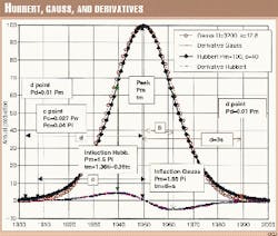
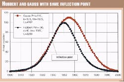
In Fig. 1, the Hubbert curve is plotted together with a Gauss curve of the same ultimate (3200), peak and peak-time. The curves are very close to each other, Gauss being a little fatter at the top and leaner at the base. The maximum of the derivative is the inflection point.
Some authorities prefer to use the following formula:
P= bU*EXP(b(t-tm)/(1+EXP(b(t-tm))2
which is equal to
P= bU/2/(1+COSH(b(t-tm))
as the cumulative production is Q=U/(1+EXP(-b(t-tm)) or Exp(-b(t-tm))=(U-Q)/Q
P = bQ-bQ2/U
The Hubbert equation is a parabola in the cumulative production (Q) domain.
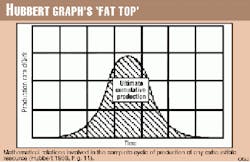
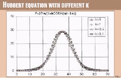
It is interesting to note that the Hubbert graph in his famous 1956 paper (Fig. 1b) has a fatter top than computed with the above formula. Hubbert did not publish a formula for the graph, and it is likely that in those days before computers he simply drew the graph by hand (with templates) and calculated the area below the curve to obtain the ultimate.
To obtain the same "fat" top as in Fig. 1b, it is necessary to add another parameter k in constructing the graph in Fig. 1c. A value of k around 0.1 (k is equal to 1 in our model) gives a similar fat top.
Procedure
The procedure for constructing the Hubbert curve depends on the status of depletion as follows:
- Post production peak. The simplest case is when the peak date (tm) and the annual production at peak (Pm) are known. All that needs to be done to construct the curve is to calculate the slope factor b by applying the formula tm-tc=c=5/b with tc when Pc=0.027 Pm. It may be further checked by making sure that b is the average of 5/c and 6/d, where tm-td=d=6/b with td when Pd=0.01Pm. The ultimate should also be equal to 0.8c*Pm. If it does not meet this check with the ultimate estimate, it probably means that the production profile has to be modeled with more than one Hubbert curve as explained below.
- Pre-production peak-post inflection. It is also possible to construct a Hubbert curve in cases where peak has not been reached by relying on the inflection point (Fig. 1), namely when the production increase reaches a maximum, but it is much less reliable. The inflection point in time (ti) and amount (Pi) corresponds with the maximum of the derivative and allows to compute:5
Pm = 1.5 Pi
tm = ti + 1.317/b = ti + 0.263c.
The production data give the amount of production (Pi) and the date (ti) at the inflection point being the maximum of Pn-Pn-1, with Pm being derived from the above equation. Thus, tc corresponds with the date when production is equal to
Pc = 0.027 Pm = 0.04 Pi; giving
c = tm - tc = 1.36 (ti-tc) and
tm = 1.36 ti - 0.36 tc.
Accordingly, Pm, tm, and c are derived from Pi, ti and tc.
The ultimate U = 0.8cPm = 1.63 Pi (ti-tc).
The cumulative production up to the inflection point is
CPi=U/(1+EXP(1.317)=0,21U or U=4,7*CPi
Applying the formula to the point d is another way to compute tm, as td (Pd=Pm/100) gives tm=1.28 ti - 0.28 td, d=1.28 (ti-td).
The same procedure can be applied in constructing a Gauss curve. The inflection point occurs for tm-ti = s and Pi = Pm*EXP(-1/2) or Pm = 1.65 Pi. The point td (where Pd = 0.01 Pm) occurs at d approximately equal to 3s. So, ti-td=2s or s = 0.5(ti-td) and U=2.5 s*Pm. The Gauss inflection point occurs sooner than with the Hubbert curve, as the curvature at the top is larger.
Although the Hubbert and Gauss curves are close, the inflection points occur at different times, so estimating the peak value from the inflection point of actual data give different values, being 1.5 or 1.65 times the inflection value. This is a substantial difference. Using the same inflection point, as in Fig. 2, Gauss peak will be in value 10% higher than Hubbert peak, and in time five years later and the ultimate 33% higher. As there is no reason to prefer one to the other (except that the Central Limit Theorem corresponds to a Gauss distribution), this difference demonstrates the uncertainty of forecasting peak on the basis of inflection point.
3. Pre-production peak-pre-inflection. Forecast cannot be made in this case because the growth is still exponential, except by the use of reserve data as follows.
3a. Using annual discovery data. Since oil has to be found before it can be produced, it is obvious that the production curve must in some degree mirror the discovery curve. Hubbert assumed a good correlation, but in fact discovery curve needs to be smoothed. In the event that discovery has peaked, it may be readily modeled with a Hubbert curve. A time shift may then be introduced to match the onset of discovery with the onset of production, so that the discovery curve serves as a proxy for the production curve. If the discovery peak has not yet been reached, the forecast becomes very unreliable.
3b. Using ultimate recovery estimates. The ultimate recovery from a natural domain, such as a basin with a single petroleum system or from many domains that combine to become a single domain, may be determined by creaming curves (cumulative discovery versus cumulative wildcats) or field size distributions (parabolic fractal). It is even possible to use the risked reserves of untested prospects as assessed on strictly geological and geophysical criteria.
In the case of a single cycle, peak is reached at the midpoint of depletion (U/2). The date of peak may then be assessed by extrapolation of the past production trend. Such an approach allows the half-life c to be computed from c = U/0.8Pm.
Applications
The foregoing explains the theory and practice of constructing Hubbert curves, drawing attention to the importance of distinguishing places with a single cycle of discovery from those with more than one cycle, which are the norm.
A set of examples illustrating how the method may be applied in practice is considered below.
1. US Lower 48
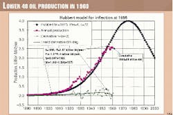
1a. US Lower 48 as estimated in 1960 prior to peak. Hubbert made his celebrated estimate in 1956 forecasting that US production would peak around 1970, as indeed it did. By coincidence, 1956 was approximately the inflection point (ti). Fig. 2 is a plot of production up to 1960 to consider how the methodology could have been applied then.
Annual production (Pi) at the 1956 inflection point (ti) was 2.67 billion bbl/year, meaning that peak (Pm) would be 1.5 times Pi, namely 4 billion bbl/year. The year that corresponds to the effective beginning tc is 1903 (Pc=0.04 Pi = 0.11 billion bbl/year). The peak time is tm=1.36ti-0.36tc=1975 and c=72.
This method, which is based on the inflection point, gives a midpoint production (Pm) of 4 billion bbl/year in 1975 and a half-life (c) of 72 years. The resulting curve is plotted in Fig. 3 and yields an ultimate of 230 billion bbl.
Using the cumulative production to inflection point in 1956 CPi=55 Gb, giving U=4.7*CPi=258 Gb, it is higher than the previous estimate because the aborted cycle by the depression.
Using a Gauss curve, with an inflection point at 1956, Pi= 2.67, Pm=1.65 Pi= 4.4 billion bbl/year, and Pd=0.04 and td= 1890, ti-td=2s, s=33, tm= 1956+33= 1990 and U=2.5 s Pm = 360 billion bbl which is unrealistic.
Taking for the sake of argument an alternative inflection point at ti=1950, Pi=2 billion bbl/year
-for Hubbert Pm=3, Pc=0.04Pm
=0.12= 1904, tm=1967, c=63, U=150 billion bbl = too low
-for Gauss Pm=3.3, Pd=0.033
=1889, s=0.5(ti-td)=30,5, U=250 billion bbl = too high.
The wide range of estimates based on unreliable inflection points is evident.
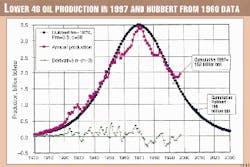
1b. US Lower 48 as estimated in 1997 after peak. Fig. 4 is a plot of annual production up to 1997 that shows a very close fit with the 1960 Hubbert model based on an inflection point occurring in 1956, save for the last three years when nonconventional oil and increasing amounts of NGL cause some departure.
It is at the same time curious to find matching shoulders in the late 1950s and early 1980s on either side of peak due to unrelated economic influences that were, respectively, proration and price rises.
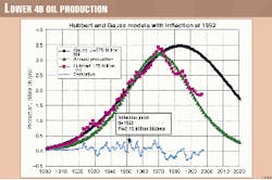
We have seen above that using the Gauss curve with an inflection point in 1956 gives an unrealistic ultimate of 360 billion bbl. As annual production varies greatly because of economic and political factors, such as the Great Depression of the 1930s and prorationing of the 1950s the inflection point cannot be easily identified. However, 1952 is the global maximum and a fair estimate of inflection. The inflection point ti=1952 and Pi= 2.15 billion bbl/year gives
-for Hubbert Pm=3.2 billion bbl/year, tc=1902, tm= 1970, c=68, U= 175 billion bbl
-for Gauss Pm=3.5 billion bbl/year, td=1889, s=31.5, tm=1983, U= 275 billion bbl.
These two different models are plotted on Fig. 5 both as could have been drawn in 1960 and with the present data. Both fit the data fairly well to 1960 but diverge afterwards, Gauss being too high and too late when Hubbert is much better. Such modeling is clearly very sensitive to identification of the inflection point, which is not easily done in practice.
Hubbert's famous 1956 effort that forecast a production peak in 1970 was based more on his knowledge of discovery and its ultimate than on the shape of the curve (or the inflection point).
1c. Discovery-production link. It is instructive to compare discovery and production curves. The US suffers from an archaic reporting practice that recognizes only proved reserves, when for this purpose we need proved and probable reserves (strictly having a mean probability), with revisions properly backdated to the discovery of the fields containing them.
Accordingly, it has been necessary to adjust the USGS6 reported annual discoveries by assuming a growth factor whereby 1 bbl initially reported becomes 5 bbl 150 years later, as based on MMS findings in the Gulf of Mexico.
Thus, for example, 1930 discovery is estimated in 1991 at 8.36 billion bbl, and the growth factor is 4.3; giving an ultimate of 9.72 billion bbl (8.36/4.3*5). Total mean discovery through 1997 works out to be 208 billion bbl based on USGS data and the MMS model. Fig. 6 shows the resulting backdated discovery pattern. A trend-line (Excel) and a Hubbert curve are plotted on the basis of a peak of 3.5 billion bbl/year in 1938 and a half-life of 70 years. Shifting the production curve by 33 years gives a remarkably close fit with the discovery curve. But a new cycle, possible from deepwater exploration, may yet arise.
2. Alaska
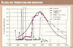
Production in Alaska comes from a small number of fields (one supergiant, three giants, and four major fields) in two separate provinces: Cook Inlet and the North Slope. These circumstances mean that Hubbert modeling should not be expected to work well.
Fig. 7 is a plot of production which, unlike in the Lower 48, is markedly asymmetrical; and there is not a good correlation between the discovery and production curves. The explanation is probably related to construction of the trans-Alaskan pipeline, which required a certain throughput before going into operation. That precluded the normal build-up of production.
A Hubbert curve could, however, be used to model the post-peak decline, assuming a 1987 peak. The respective estimates for 2010 and 2020 are Hubbert 0.1 and 0.03 billion bbl/year; DOE 0.27 and 0.17 billion bbl/year; and State of Alaska 0.27 and 0.1 billion bbl/year.
A second cycle, or the addition of natural gas liquids and synthetic oil from gas, could of course change the picture, but production from the North Slope will end when the pipeline is shut, possibly when production has fallen below 0.1 billion bbl/year. Cumulative production to 1997 is 13 billion bbl, and the cumulative Hubbert to the close of production is 4.3 billion bbl, giving an ultimate of 17.3 billion bbl.
The ultimate for US Lower 48, as estimated above, is 190 billion bbl, giving an ultimate for the US as a whole of around 210 billion bbl. Bartlett2 using a single Gauss curve gives a best fit of 222 billion bbl, which is not too far from our estimate.
3. Former Soviet Union
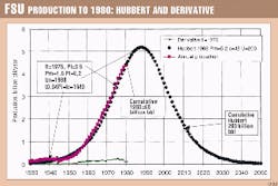
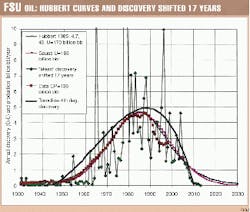
3a. FSU as estimated in 1980 prior to peak. Fig. 8 shows production from the FSU up to 1980, which totaled 68 billion bbl. The derivative curve shows an inflection point (ti) in 1975 at 3.5 billion bbl/year (Pi). Accordingly, peak production should be 5.2 billion bbl/year (1.5*3.5 =5.2). The c point is at 0.14 billion bbl/year in 1940 and the peak at 1988. The cumulative total (ultimate) from the Hubbert curve is 200 billion bbl. From CPi, U=4.7*47=220 Gb, which is higher than the previous estimate because the aborted cycle by the war.
It is interesting to note that the derivative of annual production, namely the growth, is much smoother than in the US 48 because there was no economic interference because the Soviet oil industry was not driven by economic criteria prior to 1990. The inflection point is accordingly more reliable than in the US, but in fact it is not enough.
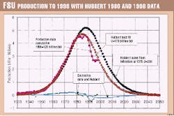
3b. FSU as estimated in 1997 after peak. Fig. 9 shows production up to 1997 amounting to 136 billion bbl, on which is superimposed the 1980 assessed Hubbert curve (U=200 billion bbl), showing a poor fit. A best fit Hubbert curve is drawn with a peak in 1985 and an ultimate of 170 billion bbl. Production was set fall under a normal decline but was exaggerated by the consequences of the collapse of the Soviet Union from 1990-95. It is now back to the level as predicted by the Hubbert curve, and set to continue to decline.
3c. Discovery-production link. Cumulative discovery for oil and condensate through 1996 was reported as 290 billion bbl, but as reserves are under-reported in the US they were over-reported in the FSU.7 Decline curve analysis of the major fields shows that their true remaining reserves are in fact approximately half as much as reported. This is confirmed by the timing of peak.
Actual peak was in 1985 when 91 billion bbl had been produced, suggesting an ultimate of about 180 billion bbl, assuming that peak coincided with depletion midpoint. Accordingly it is necessary to reduce FSU discovery to 190 billion bbl to obtain its mean discovery, about two-thirds of its reported value. Fig. 10 shows a close match between the "mean" discovery (oil & condensate) and production curves after a shift of 17 years. Note that the Gauss curve is very close to the Hubbert curve.
The US 48 and FSU are good examples of countries with a single cycle discovery, which is well modeled by Hubbert curves. But most of countries display multi-Hubbert curves.
4. UK
4a. UK-first cycle: discovery and production as estimated in 1990. The UK is sometimes quoted by detractors of Hubbert modeling as an example of a country where it does not work.
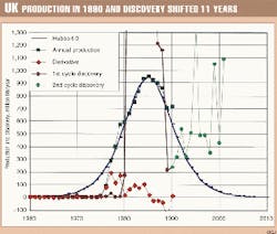
In the UK an early peak in 1990 was followed by a saddle and an unexpected second peak. In fact, there were two discovery cycles that may be satisfactorily modeled with the multi-Hubbert approach.
The first cycle of discovery peaked in at 0.9 billion bbl/year in 1974. A second discovery cycle followed with a peak of 1.3 billion bbl in 1984.
Fig. 11 is a plot of the two cycles with a good correlation between the discovery and production curves with a shift of 11 years. It clearly indicates that a second production peak was already developing by 1990. The rapid rise at the end of the 1970s obscures the natural inflection point, which cannot accordingly be used for modeling. The explanation is that whereas onshore production can start with the first well, offshore production rises rapidly once the facilities have been installed. In the case of the UK, several giant oil fields had been discovered after the opening of North Sea grabens in 1968 and were placed on production more or less simultaneously ten years later.
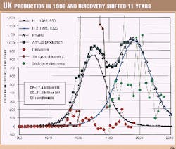
4b. UK second cycle: discovery and production as estimated in 1998. The 11-year shift between the discovery and production curves (Fig. 12) fits well with the present status of production: 17.4 billion bbl of oil and condensate have been produced so far, and 31.2 billion bbl have been discovered, of which 5.1 billion bbl is yet to be developed. The model shows clearly that production is now close to peak and will be in decline by 2001.
Fig. 10 shows modeling with two Hubbert cycles peaking in 1985 and 1998. The inflection point for the second cycle was in 1994, but as in the case of the first peak, the rise offshore is too sharp (772 million bbl/year in 1993), so it is better to take it at the average 1993-94, namely 873 million bbl/year. The value of the first cycle decline should be removed (100), so the second peak should be around 1015 million bbl/year (775*1.31). In fact, a good fit for the second Hubbert curve is 1,025 million bbl/year for 1998. Production from the first cycle will be almost exhausted by 2000, and the second cycle will be approaching exhaustion by 2010. A new cycle could arise in frontier offshore areas to the west.
5. World production
In 1974, Hubbert modeled world oil production with a low curve based on an ultimate of 1,350 billion bbl (peak at 24 billion bbl in 1991) and an high curve of 2,100 billion bbl (peak 37 billion bbl in 2000).
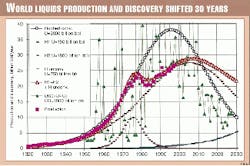
The present liquids production is plotted on Fig. 13 with a Hubbert curve with an ultimate of 2,000 billion bbl (1,800 for oil and 200 for gas liquids). It is drawn to match production to 1973, when OPEC embargoed shipments. This Hubbert curve shows what production would have been but for OPEC's prorationing, having a peak in 1996 at 38 billion bbl/year. The inflection point would have been at 1979. Obviously, the oil shock of 1973 upset the production trend, and accordingly it is not possible to draw one Hubbert curve for present world oil production.
To make a correlation with discovery, we have corrected the world database (Petroconsultants, USGS, and Canadian data) in order to obtain the mean values (about P50) for oil and condensate. Cumulative discovery is about 1,800 billion bbl including undeveloped fields. The annual discovery curve was shifted by 30 years to fit the annual production curve prior to the oil shocks of 1970s. The discovery fits well with the unconstrained Hubbert.
In addition, we have tried to model present production with several cycles: H1 for the peak of 1979, H2 for a second peak of conventional liquids, based on a combined ultimate 2,000 billion bbl, made up of 1,800 billion bbl for oil and 200 billion bbl for NGL. We have added a third cycle for unconventional oil with an ultimate of 750 billion bbl.8 The sum of these three cycles is fitted to the present data. Our forecast is that the liquids production will peak before 2010. Our previous forecast of 1998 referred to conventional oil only. Accordingly, production in 2020 would be a little less than now.
6. US population
In the mid-1920s, Pearl and Reed modeled US population with the logistic curve (termed Verhulst-Pearl) and predicted the maximum at less than about 200 million. The Hubbert modelling technique is the derivative of the logistic curve and should give better results because population can decrease.
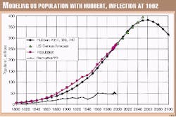
Using Hubbert modeling and the inflection point in 1992 when maximum growth occurred when the population was 255 million, the peak could be forecast at 380 million (1.5*255). Taking Pc at 10.2, tc is 1,810, and c is 247, giving the peak date tm in 2,057. A good fit is provided by taking a tm of 2,040, a Pm of 330, and a c of 240 (Fig. 14). It is obvious that Pearl in the 1920s could not achieve a good forecast because the maximum growth had not yet been reached. But in the 1930s the Great Depression interrupted the growth of population, and the present curve is lower than before.
We have plotted the US Bureau of Census forecast which is higher, as the bureau predicts about 400 million in 2050 compared with our forecast of only 330. But the bureau forecasts an unrealistic fertility rate in 2050 of 2.25 children/woman against 2.0 for Mexico, 2.02 for India, 1.3 for France, and 1.6 for Canada.
7. World population
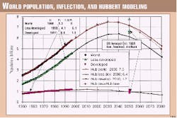
As demonstrated in an Oil & Gas Journal article (OGJ, Feb. 1, 1999, p. 57) world population can also be well modeled by summing three Hubbert curves representing respectively the industrialized world, the developing world, and a "basic" world lacking birth control.
Fig. 15 illustrates the application of the inflection point method both to the first two groups and the world as a whole, based on UN statistics (data on the third group are not available). The inflection points are 1990, 1990, and 1957, respectively.
The timing (ti) and population sizes (Pi) at inflection suggest a peak at 1.5 times the inflection population (Pi). But taking a higher peak or a Gauss curve gives a better fit. Table 1 shows the Hubbert values.
Hubbert curves have been drawn separately for the two subgroups and the world. The sum of the developed and less developed is identical with the world curve up to 2050 and diverges only slightly thereafter.
The 1998 UN forecasts of population in 2050 are classed as medium, medium-low, and low cases. The Hubbert study supports the medium-low finding. The UN forecasts for less developed countries are 6.5, 6.7, and 7.7 compared with 6.2 from the Hubbert method. For the developed countries the numbers are 0.9, 1, and 1.15 compared with 1 from Hubbert.
In other words, the Hubbert technique agrees with the UN forecast for 2050 in respect to the developed countries and is within 8% of the UN forecast for the other countries. In fact, the UN has successively reduced its forecasts since 1990, which was the inflection point when population growth reached a maximum of 90 million/year. It suggests that its forecasts are coming into line with results of Hubbert modeling.
Conclusions
Hubbert's modeling technique has been variously applauded and criticized, but the constraints to its application have not been widely appreciated.
It works well only where applied to a natural domain, unaffected by political or significant economic interference, to areas having a large number of fields, and to areas of unfettered activity. Hubbert himself worked primarily on the US Lower 48, which had the necessary characteristics to be well modeled by a single cycle.
We may note in passing that many other natural phenomena follow a bell-shaped curve. However, the application of multiple Hubbert curves, which was not developed by Hubbert, has much wider application and has proved to be an exceedingly valuable modeling tool not confined to the oil industry, as population studies confirm.
Hubbert modeling gives fair results only when the past data series has not been disturbed by economic and political factors and when the inflection point has been passed. Good results are achieved only when the past data series has passed the peak and when there is one single cycle for discovery.
The procedure of relating the discovery curve with the subsequent production curve after a time shift of a certain number of years is an indispensable tool to obtain a reliable forecast on production. The discovery curve itself, which is commonly volatile, needs to be smoothed. The time-lag is of varying duration. It is 33 years for the US; 11 years for the UK 17 years for the FSU; and about 30 years for the world as a whole, although affected by the impact of the Middle East swing producers. This shift gives a reliable trend for coming production except in the unlikely event that a major new cycle of discovery arises.
There is no doubt that Hubbert modeling is a valuable tool, but like all tools it needs to be used properly for the right job. It is important to understand its strengths and weaknesses and to know when to apply single or multicurve approaches. Knowing backdated annual discovery is a must, but it has to be the annual discovery-based mean, not proved reserves. Hubbert's model derived only from production data is an insufficient tool.
Acknowledgment
Thanks to IHS/Petroconsultants for allowing use of data.
References
- Hubbert, M.K., 1974 "On the nature of growth," 1974, http://www.technocracy.org/articles/hub-gro.html
- Bartlett, A.A., "An analysis of US and world oil production patterns using Hubbert-style curves," Mathematical Geology, 1999.
- McCabe, P.J., "Energy resources-Cornucopia or empty barrel?," AAPG Bull., Vol. 82, No. 11, 1998, pp. 2110-34.
- Laherrere, J., "World oil supply-what goes up must come down: when will it peak?," OGJ, Feb. 1, 1999, pp. 57-64 and in OGJ Letters Mar. 1, Mar. 15, and Mar. 29, 1999.
- Al-Fattah, S.M., and Startzman, R.A., "Analysis of worldwide natural gas production," SPE 57463, 1999.
- Attanasi, E.D., and Root, D.H., "The enigma of oil and gas field growth,"AAPG Bull., Vol. 78, No. 3, March 1994, Table 1.
- Khalimov, E.M., "Classification of oil reserves and resources in the Former Soviet Union," AAPG Bull., Vol. 77, No. 9, 1993, p. 1,636.
- Perrodon, A., Laherrere, J., and Campbell, C.J., "The world's nonconventional oil and gas," Petroleum Economist, March 1998, 113 p.
The Author
Jean H. Laherrère is a petroleum consultant residing in Paris, France. He retired in 1991 after 37 years with Total CFP and subsidiaries. He participated with Total in the discovery of supergiant Hassi Messaoud and Hassi R'Mel fields in the Algerian Sahara and also explored Australia, the Labrador Sea, and Michigan. He was a member of the Ocean Drilling Program safety panel. He was graduated from Ecole Polytechnique and Ecole Nationale du Petrole. E-mail:[email protected]
