Neural network identifies hidden oil, gas reserves
John D. Grace
Scott Morris
Tony Dupont
Earth Science Associates
Long Beach, Calif.
A multilayer perceptron (MLP) neural network identifies bypassed pays in existing wells. These accumulations are smaller than in typical discovered reservoirs, but can be developed faster, at lower cost, and with less risk than drilling new wells, especially considering additional transportation and processing required in new exploitation areas.
MLP machine learning
Drilling and reservoir parameters, missing sections of well logs, and optimized production strategies typically are predicted through analysis of a few neighboring wells. Machine learning, however, has not yet been fully exploited to analyze thousands of wells and hundreds of reservoirs together to gain strategic and site-specific inferences.
To address this, MLP models were applied to well logs from 5,217 wells in the Gulf of Mexico to discover untapped reserves. Using up to 10 geophysical, geochemical, and lithologic logs as inputs, predictions were made of the probability of pay (Pr(pay)) for more than 35 million 1-ft intervals in these wells. Hundreds of bypassed oil and gas accumulation candidates were discovered and subsequently filtered using engineering and economic criteria.
This approach does not replace analysis by petrophysicists and geologists but screens massive data volumes automatically, objectively, and quickly. The MLP predictions rank prospects and prioritize expert analysis. Once put in an engineering and economic context, this technology sets benchmarks for broad portfolios of opportunities.
MLP application
The wells used in the study were drilled since 2002. Of them, 2,664 produced oil and gas from 4,534 completed intervals (i.e., pays). The remaining 98% of the penetrated rock has been unproductive to date. Inputs came from up to 10 well log curves for each well. Experiments with different combinations of logs led to three classes of MLPs. Class 1 contained only three curves: measured depth (MD), deep resistivity, and gamma ray. Class 2 added two more: neutron density and bulk density. Class 3 had all 10 logs, bringing in methane, ethane, propane, and both percent sand and percent shale from mud logs. In addition to the logs, every 1-ft observation had a pay designation. If the interval falls within a completion, it is assigned a value of 1 (pay observation), otherwise it is assigned a value of 0 (dry observation).
Although different variants were tested in each class, all models had the same objective: predict pay vs. dry for each foot with the highest empirical accuracy. This is done by the MLP neural network applying a progressive series of linear and nonlinear transformations to each 1-ft log reading. In the last step it produces an estimate of probability between 0 and 1 that the 1-ft interval is in a completed pay interval. The model-estimated Pr(pay) is subsequently subtracted from the actual interval-based binary pay-dry value for that foot to produce a magnitude prediction error between model and reality. Thus, the MLP incorporates “supervised learning” architecture, where during model training each estimate is checked against reality.
The error for an interval’s prediction is then distributed back across the transformations that resulted in the prediction. On that basis, small adjustments are made in the transformation parameters to improve the likelihood that the prediction for the next observation will be closer to correct. As there are typically hundreds of thousands to millions of 1-ft observations, these small improvements accumulate, ultimately generating reliable forecasts.
After determining the best version of the models in each MLP, they were run against all intervals that had the required logs. This produced one to three predicted Pr(pay) scores for each of the 35 million 1-ft observations in the 5,217 wells. It took roughly 2-man months to analyze these wells using MLP, significantly saving time over hand analysis.
Results
Modelling with 10 log curves as input (Class 3) produced better pay vs. dry estimates than modelling with five curves (Class 2), as expected. Likewise, Class 2 modelling is more accurate than Class 1. Using a 50-50 ratio of pay vs. dry intervals to sample prediction accuracy, the best Class 1 model correctly identified pay intervals with 76% accuracy. Class 2 achieved 87% accuracy, and Class 3 recorded 97% accuracy. Increasing accuracy, however, comes at a cost.
Full log suites are not run on all wells. A Class 1 model, relying only on MD, resistivity, and gamma, will apply to 93% of all wells logged. Adding neutron density and bulk density for Class 2 reduces applicability to only 56% of logged wells. The best, most informed model, requiring 10 curves, can only be run on 6% of all logged wells. Class 3 is more applicable to deepwater wells, where logging is more extensive.
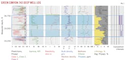
Fig. 1 shows how the models react to known productive pay in a completion interval (blue) for a well in Atlantis field (Green Canyon 743). Predictions of Pr(pay) for the three model classes are in Track 1; a black dashed line marks the candidate threshold at Pr(pay) = 0.90. The completed interval is shown in shades of blue in the center of the log. The purple lines in the context track (Track 7) show the vertical extent of the five individual completions. Track 6 shows how the average of the three model predictions follows the lithology trend (percent sand and percent shale from mud logs).
Class 2 and 3 scores clearly indicate prospectivity (Pr(pay) ≥ 0.90) in the shallowest part of the completion (Interval B). The same score occurs in the deep section of the completion interval (Interval D). In between, in Interval C, lower average Pr(pay) scores and lower coherence among them identify a heterogeneous section with poorer prospectivity log indicators.
Above completion (Interval A), none of the models exceed Pr(pay) = 0.90. Just below the completion (Interval E), there is a small prospective section identified by the Class 3 model reflecting the general practice of completing above the gas-water contact. Such zones can be easily filtered.
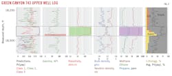
Fig. 2 shows thick, but otherwise typical, bypassed pay sitting in a shallower interval in the same well as Fig. 1. The intervals for each model’s prediction of Pr(pay) ≥ 0.9 are tinted: red in Track 2 for Class 1, green in Track 3 for Class 2, and purple in Track 5 for Class 3.
The shallow section immediately above Interval B (in Interval A) shows similar results of the log-analysis process. All three model classes condemn this section with scores of Pr(pay) < 0.90. The strength of that judgement is also proportional to the information available to each model. For Class 1, the least-informed model, Pr(pay) scores are 0.5-0.6. The better-informed Class 2 score is systematically lower, between 0.3-0.5. The negative results for the most data-intensive model, Class 3, are clear, with single-digit scores hugging the left axis.
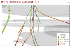
To place model results within geologic context, Fig. 3 shows Pr(pay) scores along well bores in Mars-Ursa field (Mississippi Canyon 807) in 25-ft averaged increments. Lower Pliocene-producing reservoirs are illustrated in semi-transparent gray. The scene center is at 11,732 ft subsea.
High- and low- prospectivity zones are identified among the producing reservoirs along the wellbores using colored pay flags. High-prospectivity zones (red) outside the reservoirs warrant consideration as extension targets or candidate bypassed pays, ready for detailed petrophysical and geologic examination.
Operational considerations, like the minimum thickness of candidate intervals and permissible gaps of Pr(pay) < 0.9 within them, are required for a tractable screening system. The threshold value of 0.9 can also be changed based on additional analysis and experience. Engineering and economic factors can be integrated to segregate opportunities: those in producing wells, those on open blocks, and access to production and transportation. Cataloging the concrete candidate bypassed pays found with this system depends on the exact qualifications imposed for candidacy, but these critically important factors are relatively easy to introduce and can be changed to test the robustness of the filtering process.
MLP application
The neural network approach is not specific to pay identification. The predicted variable could be gas-oil ratio, estimated ultimate recovery, or maximum production rate/ft. Such a suite of tools could assess large portfolios within companies. Alternatively, extensive regional analysis is accessible using public data, as was done in this study.
On a finer but related scale, systematic study of thousands of completions could relate the character of reservoir heterogeneities, such as that identified in Fig. 1, to completion production performance. Alternatively, mechanical logs can be analyzed to relate drilling time and costs. In such a screening analysis, most initial candidates will not justify development. However, after imposing basic engineering and economic criteria, there are still scores of promising candidates that justify expert examination.
The authors
John D. Grace ([email protected]) is president of Earth Science Associates, Long Beach, Calif. He holds a PhD (1984) in economics from Louisiana State University. He is a member of the Society of Exploration Geophysicists, Society of Petroleum Engineers, and the International Association for Mathematical Geosciences.
Tony Dupont ([email protected]) is chief operating officer of Earth Science Associates, Long Beach, Calif. He holds an MA (2009) in geography from California State University, Fullerton.
Scott Morris ([email protected]) is a mathematician at Earth Science Associates, Long Beach, Calif. He holds an MS (2012) in applied mathematics from California State University, Fullerton.


