MODELING GULF OF MEXICO LOST PRODUCTION–4 (Conclusion): Meta evaluation helps model lost Gulf of Mexico output
Valuing lost production from destroyed structures is an important measure in investment decision making, since if the value of future production is less than the expected redevelopment and cleanup cost, then the decision to redevelop the property will either be postponed or not undertaken.
In the final part of this series, we present a meta-model framework to quantify the quantity and value of lost production from the 2004-05 hurricane seasons.
Previously, in Part 3, we presented sensitivity graphs and similar charts to illustrate the manner in which system parameters impact the model output. In Part 4, we describe the use of a more sophisticated, and in many respects, more useful technique to explore sensitivity analysis and the complex interactions of assumptions on model output. We illustrate the technique with examples.
Model formulation
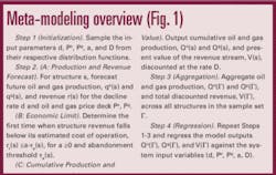
The meta-model methodology follows the basic development in Part 2 but with important structural differences (Fig. 1).
null
STEP 1: Initialization
The user selects the variables of interest and quantifies the manner in which they vary. This involves choosing the model variables, distribution functions and parameters.
The input set is user-defined and varies with the objectives of the analysis and the problem formulation. The distribution of each input variable is largely a design choice.
We employ the following variables: the price of oil and gas (Po, Pg), the threshold multiplier a, and the discount rate D. The decline curve parameter d for structures that do not yield a best-fit curve is also a model input. The input parameters are denoted by the vector (d, Po, Pg, a, D), although we also use the notation (X1, X2, …, Xn) to indicate the general nature of the model variables and the fact that their specification is both user-defined and problem specific.
Parameter Xi is governed by distribution function fi, i = 1, …, n. The specification of the function may be determined by empirical analysis or by user preference.
For example, if the historic price of oil is determined to follow a lognormal distribution according to the parameters µ and σ2, Po ~ LN(µ, σ2), the user may model future prices according to this distribution or may prefer to assume some other distribution type, such as the uniform distribution, Po ~ U(a, b).
Our preference is to maintain reasonable assumptions and bounds on the function parameters, recognizing that problem tasks and individual bias allows for a wide range of variation.
STEP 2a: Production and Revenue Forecast
The model curves for each structure are used to forecast future oil and gas production under the assumption of stable reservoir and investment conditions.
The production forecast for oil and gas begin in the year 2006 (t = 1) and continue into the future as qi(s) = (q1i, q2i, …).
Revenue in year t for structure s is computed as rt(s) = qto Pto + qtg Ptg, where Pto and Ptg represent the average oil and gas price of the production sold during the year t. We assume a price deck that is constant throughout the life cycle of the structure.
The revenue forecast vector for structure s is denoted as r(s) = (r1, r2, …).
STEP 2b: Economic Limit
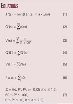
To terminate the production and cash flow vectors determined in Step 2a, we estimate the time the structure is no longer commercial by comparing the revenue each year, rt(s), to the economic limit of the structure, τa(s), and selecting the first year (earliest time) when revenue falls below the economic threshold given by Equation 1.
The value of a in Equation 1 is used to provide operational insight on the effect of changes in the threshold level. Ta(s) denotes the time when production is no longer commercial. At time t = Ta(s), the operator is assumed to stop producing, which will terminate the cash flow vector: r(s) = (r1, r2, ..., rTa(s)).
STEP 2c: Cumulative Production and Discounted Revenue
The cumulative lost production Qi(s) and discounted cash flow V(s) associated with structure s is computed from 2006 (t = 1) through the time of abandonment, t = Ta(s), as given by Equations 2 and 3.
The value of D used in the valuation computation denotes an industry-wide discount rate that is employed for each structure.
STEP 3: Aggregation
The model output for structure s is the forecast production profile, qi(s), cumulative production, Qi(s), and discounted cash flow, V(s).
We perform the assessment for each structure and then aggregate across the collection of all hurricane-destroyed structures Γ, yielding Equations 4 and 5.
STEP 4: Regression Analysis
The model input are the parameters (d, Po, Pg, a, D) and the model output includes {qi(Γ), Qi(Γ), V(Γ)}.
In the first loop of the process, each input parameter (d, Po, Pg, a, D) is sampled from its respective distribution; intermediate calculations on production forecasting, abandonment, cumulative production and discounted revenue are performed for each structure; and then the structure results are aggregated to obtain {qi(Γ), Qi(Γ), V(Γ)}.We repeat this process p times, each time resampling from the parameter distributions, performing the intermediary calculations, and compiling the aggregate results.
The final step of the analysis is to regress the model output {Qi(Γ), V(Γ)} against the input parameters (d, Po, Pg, a, D) and derive linear relations of the form shown in Equation 6, for f ∈ {Qi(Γ), V(Γ)} and (X1, X2, X3, X4, X5) = (d, Po, Pg, a, D).
The model coefficients αi, i = 0, …, 5, are determined from the regression analysis and determine the magnitude and direction of the function relative to changes in the parameter set (d, Po, Pg, a, D). The coefficients αi, i = 0, …, 5, vary with the choice of output metric f, distribution function fi, and sample size p.
Model structure
Model specification
The linear model specified in Equation 6 relates the cumulative production and present value to the model input variables.
The “proper” sign of the function coefficients αi, i = 0, …, 5 are suggested by economic theory and the model framework and provide an initial check on the veracity of the model structure.
Expected signs
The coefficient α0 represents the fixed term (intercept) of the functional and there are no expectations on its sign. Depending upon the model type and user preference, the fixed term coefficient may be excluded from the formulation.
The coefficient α1 is associated with model parameter d, which defines the rate of decline of production for those structures that have less than 7 years production history or did not yield a best-fit decline curve. The value of d will therefore “control” only that portion of annual production associated with young structures or where curve fitting was not successful.
As d increases, production at each structure will decline faster and reach its economic limit sooner, and so the quantity of reserves and their value will also decline. We would expect α1 <0 for the Qo, Qg, and V functionals because increasing d will lead to declining cumulative production and value.The coefficients α2 and α3 are associated with the price of oil and gas, respectively. As Po and Pg increase, revenue will increase, delaying the onset of the economic limit of each asset.
This in turn promotes the production of additional reserves, which at an elevated price level, will lead to a greater discounted cash flow. Thus, increasing (decreasing) Po and-or Pg will lead to increases (decreases) across all the outputs Qo, Qg, and V, and so we would expect α2, α3 >0.
The coefficient α4 is associated with the multiplier a which is used to vary the economic threshold τa. The variable a ranges over a positive interval, and as a increases, the value of a·τa(s) will increase, forcing production out of profitability at an earlier time. This will reduce cumulative production, Qo and Qg, and the value of production, V. The coefficient α4 is expected to be negative for Qo, Qg, and V.
The coefficient α5 is associated with the discount rate D that is used to compute present value, and thus, will only influence the valuation estimate V. The behavior of discount rate with present value is well known: as D increases, the value of future cash flow declines, and so we expect the sign of the coefficient α5 to be negative. Coefficient α5 is not included in the model specification for cumulative production.
Function interpretation
The functional construct is used to compute the expected value of the output for any parameters that fall within the design space, as well as to investigate the impact of one or more changes in the input parameters on the model output. The functional represents the average relation between the input variables and model output for the input parameters specified, and thus the model coefficients must be interpreted with respect to the geometry of the design space (Fig. 2).
Model summary
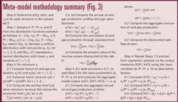
A summary of the model structure is provided in Fig. 3.
Model resultsDesign space
The parameters and distribution functions that serve as model input are shown in Table 1.
These parameters lead to a four-dimensional hypercube design space, shown in Equation 7, where the oil and gas price distributions are truncated at two standard deviations.
Cumulative lost production
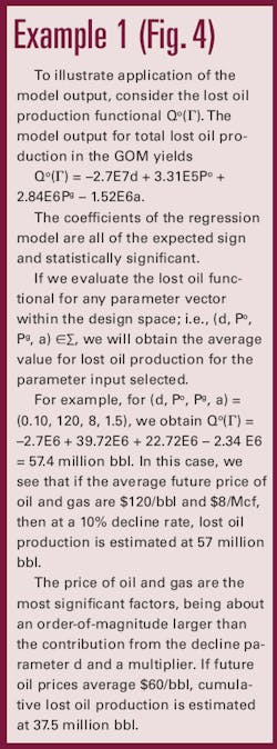
Following the modeling steps described above, regression models for cumulative lost oil, gas, and BOE production are constructed as shown in Table 2. In Fig. 4, an illustrative example is provided.
null
Valuing lost production
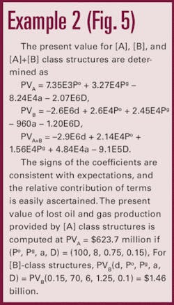
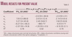
Present value functionals for the oil and gas stream forecast is shown in Table 3 for [A] and [B] class structures, where [A]-class structures denote normal assets and [B]-class structures denote young and chaotic producers. Fig. 5 provides an example.
null
Acknowledgments
The advice and critical comments of Kristen Strellec are gratefully acknowledged. This article was prepared on behalf of the US Department of the Interior, Minerals Management Service, Gulf of Mexico OCS region, and has not been technically reviewed by the MMS. The opinions, findings, conclusions, or recommendations expressed in this article are those of the authors, and do not necessarily reflect the views of the Minerals Management Service. Funding for this research was provided through the US Department of the Interior and the Coastal Marine Institute, Louisiana State University.
The authors
Biographies for coauthors Mark Kaiser and Yunke Yu were published in part 1 of the series (OGJ, July 7, 2008, p. 42).
Christopher J. Jablonowski is an assistant professor in the Department of Petroleum and Geosystems Engineering and associate director of the Energy and Earth Resources Graduate Program at the University of Texas at Austin. Before joining UT in 2005, he worked as a consultant with Independent Project Analysis Inc., as a senior drilling engineer and buyer with Shell Oil Co., and as an energy economist with the US government. His research interests lie in value of information and decision-making under uncertainty, HSE performance assessment, and qualitative response models and detection-controlled estimation. He has a PhD in energy, environmental, and mineral economics from Penn State University.
